
Recently I needed to find the maximum and minimum of a range of values including some #N/A values. Searching found a variety of solutions, of which the simplest (that works in all versions) seems to be:
- =MAX(IF(ISNUMBER(datarange),datarange))
- =MIN(IF(ISNUMBER(datarange),datarange))
The function must be entered as an array function, i.e. type the function, then press Ctrl-Shift-Enter, rather than just Enter. The screenshot below shows a simple example:
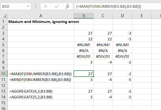
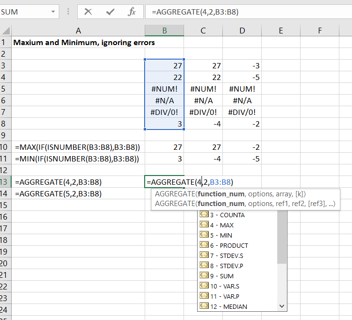
The search also found the Aggregate function, which is new in Excel 2010, and provides a number of options for ignoring sub-totals as well as errors. The Aggregate function will return a number of different statistical functions, as well as Max and Min. These are documented with a tool=tip as the function is entered, as shown in the screen-shot below:

Pingback: More on Sums | Newton Excel Bach, not (just) an Excel Blog
You have not quite yet perceived the power of the aggregate function. It is huge when you see past the simple applications.
Where it is most valuable is to find the max, min, percentile median etc of filtered lists.
What is the median of all values in column A that have a 1 in the corresponding position of column B. or which have a 1 in column B AND the word ‘here’ in column C etc.
There are some nice and well documented ways to find means in such situations using the sumproduct() ie
Mean(A1:A100 such that B1:B100=1) = sumproduct(A1:A100,N(B1:B100=1))/ sumproduct(N(B1:B100=1))
But this does not work for medians etc..
However this does:
=AGGREGATE(16,6,(A1:A100)/(B1:B100=1),0.5)
This corresponds to using function number 16 (percentile inclusive) with a percentile target of 0.5 (the median) and ignoring all errors (code=6). Any cell in B1:B100 that contains a 1 will divide the adjacent A value by 1 (ie leaves it alone) while any value that is not 1 will code as a zero and will produce a divide by zero which will be ignored by the aggregate().
Change the final argument (0.5) to a zero and you will get the minimum of the selection, set it to 1 and get the maximum. and set it to any other value and get the corresponding percentile.
You can use a very similar construct to find the nth smallest or largest of a selection using functions 14 or 15 respectively and appropriate targets in the last argument.
You can extend the number of conditions by dividing by further conditional statements
It really works!
Note that for reasons that maybe some low level coder at Microsoft only knows, the Min and Max versions (function 4 and 5) do not work unless they are coded as array functions.
This seems an undocumented feature that I love!
Bob Jordan
Excel Nutter!
LikeLike
“You have not quite yet perceived the power of the aggregate function”
Give me a chance, I only found it last week! 🙂
But thanks for the comments, and I’ll certainly give it a closer look.
LikeLike
I’ll echo Doug’s “give me a chance” comment…and his gratitude for being pointed in a direction, akin to someone saying: “Sure that mountain looks great from here, but wait till you climb it – the view from the top is unbelievable!”
Aggregate() appears to be that peak that’s just calling to be climbed. But the task before me now is to begin the exploration.
LikeLike
I was at the Modeloff conference in London recently, and I was manning the Excel desk. One of the questions asked of me was how to produce a sum of values in a column with a condition, but exclduing any columns hidden by a filter. Using a simple example similar to (the other) Bob’s, values in A2:A10, and a flag of 1,2,3 or 4 in B2:B10, sum A2:A10 where B2:B10 is 1 or 2, but exclude hidden rows.
My nitial thought was to use my old tried and trusted SUMPRODUCT
=SUMPRODUCT((B2:B10={1,2})*(SUBTOTAL(103,OFFSET(INDEX(B2:B10,1,1),ROW(A2:A10)-ROW(INDEX(A2:A10,1,1)),0)))*(A2:A10))
I then though of using AGGREGATE to create a helper column identifying the hidden rows
=AGGREGATE(2,5,A2)
and sum the two conditions with SUMIFS
=SUMIFS(A2:A10,B2:B10,1,C2:C10,1)+SUMIFS(A2:A10,B2:B10,2,C2:C10,1)
This worked, and I could have used one SUMPRODUCT rather than two SUMIFS, but seemed klunky to me.
Next, I tried to use AGGREGATE to do it all in one step
=AGGREGATE(9,5,(A2:A10)*(B2:B10={1,2}))
but that just gave me an error, even with all rows visible.
I summised that AGGREGATE wouldn’t sum the array returned, so I tried another approach, use AGGREGATE to return an array and sum that
=SUM(AGGREGATE(14,7,(A2:A10)*(B2:B10={1,2}),ROW(A2:A10)-ROW($A$2)+1))
I had to array-enter it, but it worked … when all rows were visible. If I filtered it such that one of my target rows were hidden, I got the same result as I did with no rows hidden. I am thinking that the array returned by this part, (A2:A10)*(B2:B10={1,2}), which still includes the hidden rows, is treated as all being visible, so all are summed.
I feel that AGGREGATE has a lot of untapped power, and I must be missing something fundamental, but I cannot hyet get it to do what I want.
LikeLike