… or at least, a non-intuitive feature of the MATCH function, that may give inconsistent results.
This post is based on a discussion at EngTips.
The problem under discussion was to find the number of the first and last rows containing data in a column, when the data was in a single block, with increasing values. The suggested formulas were:
- Start: =MATCH(TRUE,C6:C157<>0,0)+5
- End: MATCH(TRUE,C6:C32<>0,1)+5
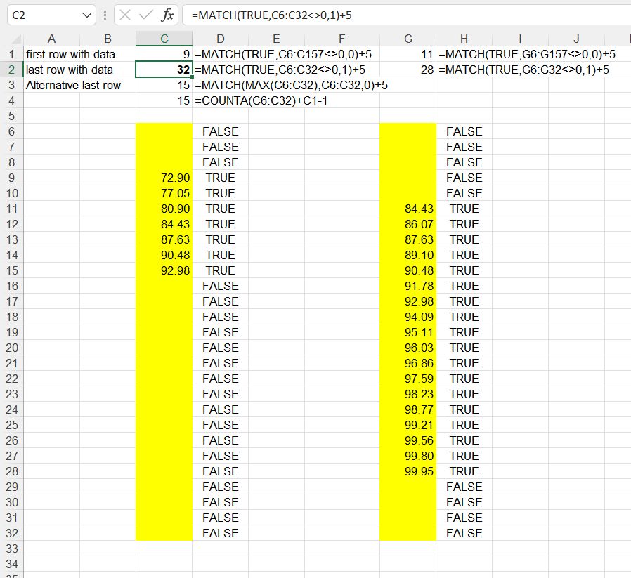
A simple example is shown below:

Note that the start and end row of the data in column G is reported correctly, and the start row is correct in both cases, but the formula for the end of the data in column C returns the end of the search range, rather than the end of the data.
Looking at the formula in more detail:
MATCH(TRUE,C6:C32<>0,1)
C6:C32<>0 returns an array of TRUE or FALSE values, as shown in columns D and H.
MATCH(TRUE,{ARRAY},1) should return the row number in ARRAY of the last cell containing a TRUE value (which is how it works in column G), but the last argument is the “match type”, with 1 indicating that the last row number with contents less than or equal to the match value should be returned. Because the data is supposed to be increasing in value the function performs a binary search. Starting at the centre of the search range, if this value is blank (and therefore less than the search value), it will check only cells further down the range, and since all these are also blank, it ends up in the last cell of the range, and returns this as the answer.
Two alternative formulas are given are shown in the spreadsheet, which will always give the correct result, provided that the data is continuous and increasing:
- =MATCH(MAX(C6:C32),C6:C32,0) + 5 (where 5 is the number of the row immediately above the search range.
- =COUNTA(C6:C32)+C1-1 (where C1 is the row number of the start of the data)
Note that the first formula will give the correct result if the data has gaps, provided that the last cell with data has the maximum value. For the second formula the data does not need to be increasing in value, but it must be continuous.

Another perhaps better or more robust approach for finding the last non-blank numeric cell could be…
=MATCH(99^9,C:C,1)
The idea is that you lie to Excel by telling it the data is sorted (which it can be but doesn’t have to be) and send it hunting for a massive number that will never be found, causing it to settle for the last row.
If the column were text instead of numeric, then this would typically be an equivalent, assuming every existing value starts with a more traditional character from the keyboard…
=MATCH(“Ω”,C:C,1)
The Ω, which can be typed using Alt+234 on the numeric keypad, is “bigger” than any character in the keyboard and is much like using “zzzzz” for the search.
And if it’s a mixed bag of text or numeric, then use…
=MATCH(2,1/(C:C””),1)
The resulting array is comprised entirely of 1 and/or #DIV/0! where the errors are ignored and the 2 (or any number higher than 1) being sought is bigger than 1, causing it to settle once again for the last non-error.
LikeLike
Thanks David, some interesting suggestions there.
With numeric data your first suggestion seems to work for any data (as long as it’s all < 99^9).
I found the last suggestion works with text within the data range, but if the last row is text then it returns the last row with a number. Also it seems to work with the search term reduced to 0.1, but for any lower value it returns the last row less than zero, which seems a bit strange.
LikeLike
I think that last formula may have somehow pasted or rendered incorrectly. There should be an equal sign between the C:C and the set of double quotes. The idea is to take the number 1 and divide it by the question of whether the cells in C are blank (or at least equal to the null string). The question results in an array of TRUE or FALSE that turn into a 1 or 0 as a result of the math and produces the set of 1 or #DIV/0! values.
LikeLike