… with Numba and Scipy sparse matrix functions.

As promised in the previous post in this series, I will be looking at speeding up the formation and solving of matrix functions for the analysis of structural frames, using Excel and pyxll to call Python routines with the Numba jit compiler, and Scipy sparse matrices and solvers.

For an example I have used the 3D analysis of a concrete building frame with 7065 beams and 2730 nodes. This has 14,742 degrees of freedom, which if analysed using the complete stiffness matrix would require creating and solving a matrix with 217,326,564 elements. The actual matrix has only 176,904 non-zero elements, so the use of a matrix in sparse format saves an enormous amount of memory resources and computing time. The use of alternative Scipy solvers, and options within each solver, also made a huge difference to the solution time.

The table below shows times for reading the data from Excel and setting up the stiffness matrix:

The time saving from using Numba is fairly modest (presumably because most of the work involves manipulating data within Numpy arrays), nonetheless the creation of the final stiffness array shows a useful time saving when using Numba.

I have used two matrix solver routines from the Scipy linalg and sparse.linalg libraries, and each of the 9 alternative iterative sparse solvers:

• solveh_banded: Solve equation a x = b. a is Hermitian positive-definite banded matrix.
• spsolve: Solve the sparse linear system Ax=b, where b may be a vector or a matrix.
• Iterative solvers:
• bicg: Use BIConjugate Gradient iteration to solve Ax = b.
• bicgstab: Use BIConjugate Gradient STABilized iteration to solve Ax = b.
• cg: Use Conjugate Gradient iteration to solve Ax = b.
• cgs: Use Conjugate Gradient Squared iteration to solve Ax = b.
• gmres: Use Generalized Minimal RESidual iteration to solve Ax = b.
• lgmres: Solve a matrix equation using the LGMRES algorithm
• minres: Use MINimum RESidual iteration to solve Ax=b
• qmr: Use Quasi-Minimal Residual iteration to solve Ax = b.
• gcrotmk: Solve a matrix equation using flexible GCROT(m,k) algorithm.

For all cases the initial “A” matrix (i.e. the square stiffness matrix) is prepared in COO format, which allows the matrix to be compiled with the minimum of calculation. The COO format consists of 3 columns listing each non-zero value of the array, and the row and column number of each value.

The solveh_banded function requires the A array to be a Hermitian banded array. Scipy does not seem to have a function to convert from COO to banded, so I wrote one:

def COO2BandedVect(kv, ki, kj):
    """
 Convert a COO matrix to symmetric banded upper triangle format.
 kv ki kj: COO matrix vectors
    """
    rows = kv.shape[0]
    n1 = 0
    cols = 0
    for k in range(0, rows):
        i = int(ki[k])
        j = int(kj[k])
        if i > cols: cols = i
        if (i-j) > n1: 
            n1= i-j
    cols = cols+1
    bandwidth = n1+1
    
    BandMat= np.zeros((bandwidth, cols))
    for k in range(0, rows):
        i = int(ki[k])
        j = int(kj[k])
        if i - j <= 0: BandMat[ i + (n1-j), j] = BandMat[i + (n1-j), j] + kv[k]
    return BandMat   

For the other functions the three vectors, v, i and j, must be converted to a COO matrix then to csc or csr format, which may de done with a single line of code:

 A = ssp.coo_matrix((v,(i,j)),shape=(n,n)).tocsc()

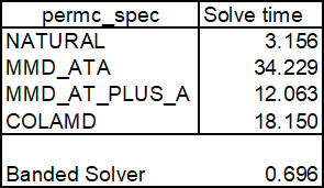
The solveh_banded function performed much better than the other analytic solver (spsolve) with default arguments, with solution times of 0.70 and 18.15 seconds respectively. Spsolve has an optional argument called permc_spec that defines “how to permute the columns of the matrix for sparsity preservation”. The options with solution times are shown below:

For this case the “Natural” option is thus almost 6 times faster than the default “Colamd” option, and 11 times faster than the slowest option! The solveh_banded function, with default arguments, however remains substantially faster.

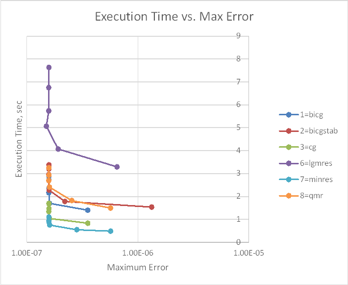
The 9 iterative solvers also had a huge range of performance, with solution times ranging from 0.5 seconds to 69 seconds. The gmres solver was by far the slowest, and gcrotmk was also very slow. The cgs solver returned an error. The performance of the other 6 is shown in the graphs below, with the first plotting solution time against the input tolerance value (log scale), and the second solution time against maximum error, compared with the results from the analytic solvers.

The minres solver was substantially faster than the others, but also generated greater errors with the default tolerance. The errors from the other solvers were all close to the minumum when run with the default tolerance of 1E-08. To reduce the minres error to this level it was necessary to reduce the specified tolerance to 1E-11. With this reduced tolerance minres remained the fastest of the iterative solvers, with a solution time of 0.75 seconds.

In Summary:

• The banded solver (solveh_banded) was the fastest overall for high precision results, when run with default input.
• The spsolve function performed much better with the permc_spec argument set to “NATURAL”, rather than the default, but was still substantially slower than solveh_banded.
• The minres function was the fastest of the iterative solvers, but required the tolerance value to be set to 1E-11 to minimise the maximum error in the results.
• All results are based on solving one large, very sparse matrix. Different problems are likely to have different functions giving the best results.