At Daily Dose of Excel Jeff Weir has been looking at alternative methods of applying the VLookup function and ways of getting precise timing of the different formulations.

Based on his posts there I have written two Lookup User Defined Functions (UDFs):

1. The LookExact Function finds the nearest lower match to a lookup value from a list of sorted data, then checks if this value is exactly equal to the lookup value (or optionally within any specified tolerance).  The advantage of this approach over using the built-in VLookup function with the “Approximate Match” option set to false is that a binary search on sorted data (as performed when the “Approximate Match” option is set to True) is hugely faster than searching through the list from beginning to end.
2. The LookNear function also   performs a binary search to find the nearest lower match to the lookup value, then checks the next value from the list, and returns the closer value.

Checking the performance of these functions revealed some surprising differences, which in some cases turned out to be more to do with the method of timing than real differences between the various formulas and VBA routines, so I have also added my own version of the timer routines published at: speed performance measure vba function.

A spreadsheet including the Lookup functions and timer routines can be downloaded from: ExactLookup.zip, including full open source code and some example timings as discussed below.

Four alternative lookup formulas, and the two UDFs are tested in the spreadsheet, as shown in the screen shot below:

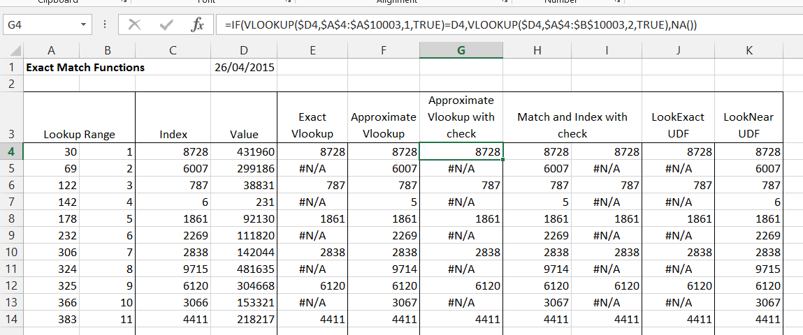
The lookup range in the download spreadsheet consists of 10,000 sequential numbers in column A, with an index value in column B.  The formulas have also been checked on a table of 1 million rows.  Column C contains 200 index values used to generate the values in Column D, using the formulas:

1. =Index(A$4:A$10003, C4)
2. =Index(A$4:A$10003, C5) + 1
3. =Index(A$4:A$10003, C6)
4. =Index(A$4:A$10003, C7) – 1

These four formulas were then copied down 200 rows to generate values that were alternately an exact value found in the lookup table, or just over or under one of the exact values.  Having generated the list the formulas were then converted to values.

Columns E to K contain:

1. E: Exact Vlookup –  =VLOOKUP($D4,$A$4:$B$10003,2,FALSE)
2. F: Approximate Vlookup – =VLOOKUP($D4,$A$4:$B$10003,2,TRUE)
3. G: Approximate Vlookup with check –
   =IF(VLOOKUP($D4,$A$4:$A$10003,1,TRUE)=D4,VLOOKUP($D4,$A$4:$B$10003,2,TRUE),NA())
4. H,I: Match and Index with check –
   =MATCH(D4,$A$4:$A$10003,1)
   =IF(INDEX($A$4:$B$10003,H4,1)=D4,INDEX($A$4:$B$10003,H4,2),NA())
5. J: LookExact UDF – =LookExact($D$4:$D$203,$A$4:$B$10003,2)
6. K: LookNear UDF – =LookNear($D$4:$D$203,$A$4:$A$10003,$B$4)

For the rows where the lookup value is an exact match to a value in the lookup range all the formulas return the same result (the index number from column B).  Where there is no exact match formulas 1, 3, 4, and 5 return #N/A, as intended.  Formula 2 returns the index number for the last row that is less than the lookup value, and Formula 6 (LookNear) returns the index number for the row that contains the value closest to the lookup value.

The screenshot below shows the input for the Timeit routine, and typical results:

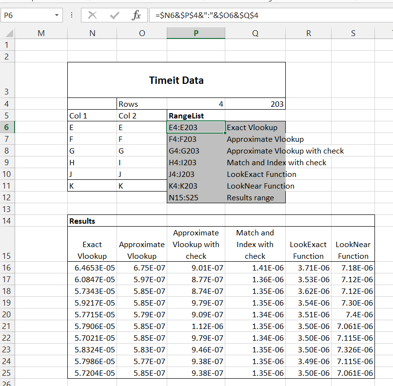
The required input is the two grey shaded columns.  The first column lists the ranges containing formulas to be timed.  Normally each range will have the same number of rows, but this isn’t necessary.  The table has been set up to generate the range addresses from the adjacent row and column details, but the ranges can also be just typed in as text.  The second column contains a description of each of the formulas.  The final row of column 1 contains the address for the output results, which should be 11 rows x one column for each formula range.

The range list may be extended (or reduced) as far as required.  If the number of rows is changed, or if the list is moved, the range name “RangeList” must be adjusted to suit.

Note that the extent of the array functions in columns J and K must be adjusted to match the recalculation ranges listed in P10 and P11.   To do this:

• Edit the first cell in each column so that the first argument (“lookval”) covers the required number of rows.
• Re-enter by pressing Ctrl-Shift-Enter.
• Re-size the array extent by pressing Ctrl-Shift-S, which calls the custom  SetArrayToNaturalSize routine.

The Timeit routine recalculates each of the listed ranges 10 times, and generates a table of recalculation times in seconds per row.  To run the routine press Alt-F8 and select Timeit.

Typical results for a range of lookup table sizes and number of functions are shown below:

It can be seen that the “Exact Vlookup” formula is by far the slowest, and with the long table it is over 7,000 times slower than the “Approximate Vlookup”.

The “Approximate Vlookup” is the fastest, but if the formula is required to return #N/A if there is no exact match, then the “Approximate Vlookup With Check” formula was surprisingly fast, taking only 25% longer on the long tables.

Splitting the formula into two columns, and using the Match and Index functions was, surprisingly, slower than the equivalent using Vlookup.

The two UDFs were slower than the Approximate VLookup formulas, but since the calculation time was only 4 to 8 microseconds, even with the 1 million row table, this would only become significant for enormous tables.