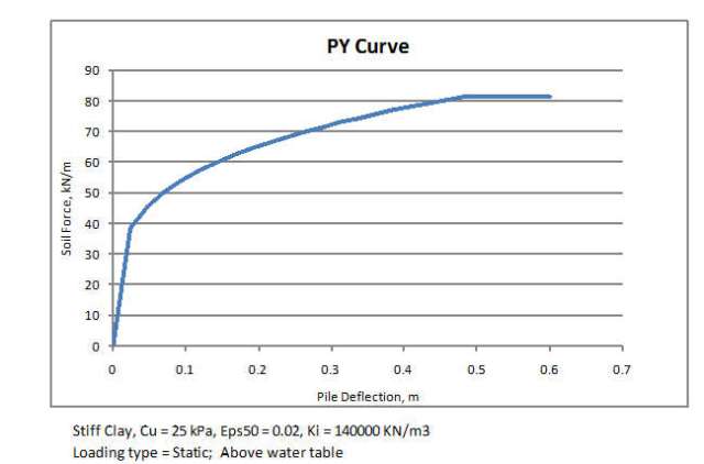
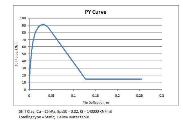
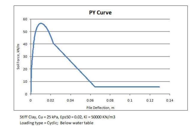
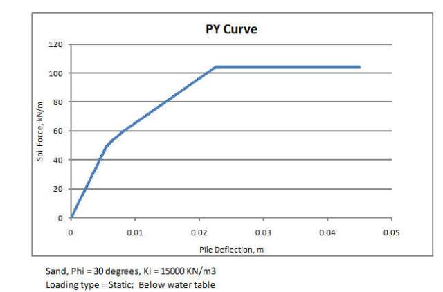
The pile lateral load analysis program presented in a previous post used linear elastic spring supports to model the restraint provided by the soil. Soil stress/strain behaviour is of course highly non-linear, and this post presents an Excel User Defined Function (UDF) that will generate non-linear force-deflection curves (often known as P-Y curves) for a variety of soil types, above or below the water table, and under static or cyclic loading. This function will be incorporated in the pile analysis program in a future post, together with non-linear behaviour of reinforced concrete piles.
The curves are based on those described in the manual for the COM 624 pile analysis program, which is available for free download from the US FHWA, together with many other valuable documents. The contents of this manual, together with other aspects of pile design, are summarised in detail in the “Theoretical Manual for Pile Foundations” published by the US ArmyEngineer Research and Development Center. The linked download site, Vulcanhammer.net, also has a wealth of other documents related to piled foundations available for free download.
A spreadsheet containing the PY624 function and examples, including full open source code, may be downloaded from PY-COM624.zip. Note that the latest version of the LatPile spreadsheet incorporates significant changes to the PY curve function, giving closer results to those in the COM624 Manual. This may be downloaded from: LatPilePY.zip.
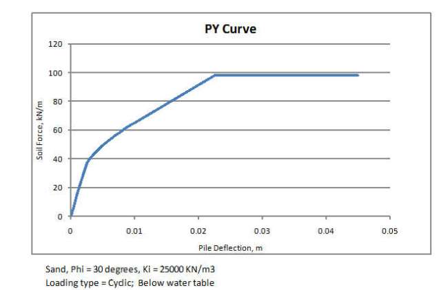
Input and output details are given in the spreadsheet, and are shown in the screenshots below, together with typical output for a variety of soil types. As always, feedback on the spreadsheet is welcome, using the comment link at the bottom of the post.


I downloaded already the excel spreadsheet PY – COM624 .ZIP, but every time that I have tried to change any input data, the program freezed, should I have to set up something before any new run?, I will really appreciate any information that you can provide, Thanks in advance for your time and consideration
LikeLike
Mario – it shouldn’t need anything other than Excel. I have just downloaded the version from my download site, and it is working on my computer. I will try it on another computer later.
Which version of Excel are you using?
Do you enable macros when you open the spreadsheet? (the message is easily missed in Excel 2007).
When you say the program freezes, do you mean you have to restart Excel, or the function results don’t change when you enter new data?
LikeLike
Doug
Once you incorporate this into the pile design you will really have something. I always struggle with COM624 input and output. I always seem to generate inputs for COM624 in excel and then take the output from COM624 and manually input into excel. It has been too much book keeping. An excel version would make my life much easier when it comes to analyzing these problems.
LikeLike
DH – see latest post: https://newtonexcelbach.wordpress.com/2010/07/17/lateral-pile-analyis-with-py-curves/
LikeLike
Pingback: Lateral pile analyis with PY curves … « Newton Excel Bach, not (just) an Excel Blog
I’m a geotech. engineer in Taiwan, I often come to this website and download your spreadsheet, thank you deeply.
According to COM624P’s manual, it just recommanded the P-Y curve fo soft clay below GW (Matlock, 1970) in Part 2, Chap. 3 (page 323), but no P-Y curve of soft clay above GW was recommanded or mention.
However, it could be found that the Appendix A (page 443)’s input variables KSOIL =2 is “for soft clay”, no mention below or above GW. I guess COM624P use Matlock’s criteria for soft clay below and above GW both. The only difference between them is the Garma of eq. 3.8 (page 324), it were Garma Saturated for above condition, and Garma Submerged for below condition. In your opinion, does that calculate in COM624P’s coding?
The other question, could you tell me the meaning of “TOTAL STRESS” column fo COM624P’s output file? Is that mean the axis stress + flexural stress due to bending moment?
Thank you very much again.
LikeLike
Qasy – I agree that Matlock’s curve for soft clay would be the most appropriate one for soft clay above or below the water table, but that is Soil Type 1, not Type 2.
Yes, I take the “total stress” to be the maximum stress combining axial load and bending (so the maximum stress in compression for a compressive axial load).
LikeLike
Pingback: Daily Download 7: Lateraly loaded pile analysis | Newton Excel Bach, not (just) an Excel Blog
Dear Doug,
First of all thank you for this amazing blog. I am learning new things from this blog each and everytime I visit!
I have a question about the p-y program: I have studied the code and method that you are using to calculate the (As) constant for static loading – stiff clay case – with presence of water. First of all the graphic does not fit the reference which is used in book (Figure 3.16 “Values of Constants As and Ac”, Single Piles and Pile Groups under Lateral Loading, Reese & Van Impe, ). Where did you get the mathematical formula for A_s constant?
And why didn’t you calculate A_c constant in the code? (The coeffeicient for cyclic loading case). is there a function to describe this value according to depth ratio (z/b) ?
Thanks in advance,
– Arif
LikeLike
Thanks for the comments and your interest.
The As and Ac factors for stiff clay are found under the stiff clay case (Case 2) in the PY function (as I think you have found).
The calculation for A_s when LoadType = “S” is for the static case, then under “Else” is the calculation for A_c, but for convenience I have used the same variable name; it would have been clearer if I hadn’t called it A_s, because it can be either, depending on the value of LoadType.
I have taken the values from Figure 3.7 in the COM 624 manual. I have just assumed a constant value of 0.6 when the depth ratio is greater than 4 for A_s, or 0.3 for Depth Ratio greater than 2 for A_c, then a parabolic distribution down to the minimum value of 0.2.
I don’t have the book you referred to, but I would be interested to know if this shows different values. The COM 624 Manual is available for free download, let me know if you can’t find it.
LikeLike
Dear Doug,
I’ve understood the calculations for As and Ac, thank you. This misunderstanding is happened to the same variable name I think.
The parabolic function that you used in your code is slightly different that the book. By the way I can send a dropbox link for the book, if you want. It can be seen if you overlap that figure into the mathematical functions’ excel graph. I don’t know how to upload an excel file into this comment section. But, as I mentioned above the difference is almost nothing. So it can be neglected I think. The questions solved 🙂
However, when I was studying on my code, I realized another thing: For static loading in stiff clay (in presence of water) while calculating the first linear part of p-y curve, you are using (ks x b) (initial stiffness * diameter) value. Shouldn’t it be depend on the depth “z” value also? What do you think?
Thanks,
– Arif
LikeLike
Arif – see:
https://newtonexcelbach.wordpress.com/2012/01/23/latpilepy-1-02/
for comment on the question of how to calculate the initial stiffness, and
https://newtonexcelbach.wordpress.com/2012/07/04/latpilepy-1-04/
for the latest version of the spreadsheet, which does the calculation the COM624 way by default, or optionally as in the original version described here.
I will update this post to link to the new file, but it’s always a good idea to look under the “Downloads by Category” menu to see if there are new posts on any subject, especially when the original is quite old.
LikeLike
Arif – I would be interested to see the book’s version of the curves by the way. You can e-mail me at dougaj4 at gmail.
LikeLike
dougaj4-What’s your email address??Can you help me a problem about p-y curve for c-phi soil??
LikeLike
Good work Doug,
Let me start by registering my opinion that your posts highly impact the humanity positively. Thanks a lot. I have just come across your Excel UDF (LatPile) for laterally loaded pile analysis. I have learnt a lot from it. However, I have a question to ask. It is a fact that the soil modulus Es for nonlinear soils vary with both depth(x) and deflection (y) that is why the literature (COM624 inclusive) mentions the following steps for solution: “(1) A set of Es values is assumed for the entire length of the pile. (2) The set of difference equations are solved to obtain the deflections at each point along the pile. (3) From the p-y curves and the values of y found in Step 2, a value of p is found at each point. (4) A new set of Es values are computed using the p and y values found in steps 2 and 3. (5) The procedure is continued until convergence is achieved.” However, in the examples presented in LatPile, only one p-y curve is used rather than using discrete curves corresponding to different depths. By this, I would assume that your LatPile code takes into account Es variation with deflection but not with depth. Could you please shade more light on this?
Best regards
Faisal
LikeLike
Faisal – have a look at https://newtonexcelbach.wordpress.com/2012/01/23/latpilepy-1-02/, which describes options for dealing with the soil stiffness varying with depth.
Also you can have as many different py-curves down the pile as required.
The latest version of the spreadsheet is https://newtonexcelbach.wordpress.com/2012/07/04/latpilepy-1-04/
Feel free to ask if anything is not clear.
LikeLike
Thanks a lot Doug. That answers my query. How would one use the LatPile to tackle other boundary conditions such as when a combination of any of the following is given: (i) lateral load and slope (e.g. fixed pile head), (ii) moment and deflection, or (iii) lateral load and rotational constraint constant (Moment/Slope)?
Thanks in advance.
Faisal
LikeLike
I downloaded the LatPilePY.zip and extracted it to have a LatPilePY.xsl, LatPilePY.xslb and 3 samples.xslb But all file are empty Excel sheets.
Can you help? Thanks.
LikeLike
I have just downloaded the zip file and everything seems to be OK on my computer.
If you e-mail your downloaded zip file to my gmail account (dougaj4) I will have a look.
LikeLike
Dear Doug.
I have downloaded already the excel spreadsheet PY – COM624 .ZIP, but every time I try to change the data, the program doesn’t work or the output numbers don’t appear, should I have to set up something before any new run?, I will really appreciate any information that you can provide, Thanks in advance for your time and consideration
LikeLike
Try this:
Extract the PY-COM624.xls file from the zip file
Right click on the file name
Click “show more options”
Click “properties”
Click the “unblock” box down the bottom.
That should fix it.
It seems to be a requirement for any downloaded file these days.
LikeLike