Following some discussion at Eng-Tips and elsewhere I have updated the LatPilePY spreadsheet, previously presented at Lateral pile analysis with PY curves …  This spreadsheet provides User Defined Functions (UDFs) to carry out the analysis of vertical piles under lateral loading, following the method described in the manual for the program COM624.  See the earlier posts for more details.  The new spreadsheet, including full open source code, can be downloaded from LatPilePY.zip .

The main change, as discussed in the Eng-Tips thread, is to the way in which the initial soil stiffness is calculated.  The soil stiffness is defined by a factor Ki which has units of Force/Length^3.  The previous version of the spreadsheet converted this factor to units of Force/unit deflection/unit length of pile by multiplying the Ki factor by the pile diameter (resulting in a factor independent of depth), whereas in COM624 the Ki factor is multiplied by the depth of the soil layer (resulting in a factor independent of pile diameter).  Both approaches clearly involve gross approximations, but to allow users to get a reasonable comparison with COM624 results I have now introduced an option to allow either method to be applied, with the COM624 method being the default (see screenshot below):

LatPile input; click for full sized view

Other significant changes are:
The calculation of the effective depth of layered soils has been amended to follow the COM624 method more closely.  Soil layers with varying strength and density affect the stiffness of lower layers in 3 ways:

1. Where the ultimate soil resistance is controlled by wedge failure the failure load is affected by all the layers through which the wedge passes.
2. Where the initial stiffness of a soil is related to the vertical pressure, this is affected by the density of the overlying soils.
3. For deeper layers, where the ultimate resistance is controlled by soil flow around the pile, the failure stress of granular soils is related to the vertical pressure.

For this reason two separate effective depths are calculated at the top of each layer:

1. The depth of soil, with the same properties as the layer, that would have the same ultimate resistance to wedge failure as the actual upper layers.
2. The depth of soil, with the same density as the layer, that would have the same vertical pressure as the actual upper layers.

These two effective depths are calculated by the program, but provision has also been made to specify override values in the Soil Properties Tables; see screenshot below:

Soil property input, including new optional effective depth rows

The other major change is that additional columns may (optionally) be added to the output array, providing details of the calculated effective depths, ultimate soil resistance, and calculated soil force/unit length of pile.

LatPile output options

LatPile output with Output Option 3 (11 columns)

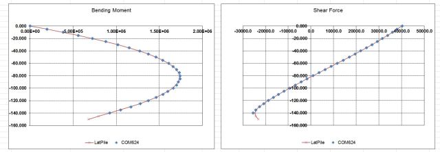
The spreadsheet results have been compared with 3 examples from the COM624 manual (full details are included in the download file). The first example is for a single layer soil, and shows very good agreement in all respects:

COM624 Example 1

COM624 Example 1

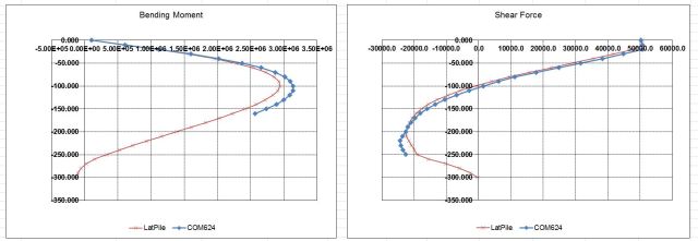
The second example is for a layered soil with varying soil types and densities.  When user defined effective depths have been used reasonably good agreement was found:

COM624 Example 2; User defined effective depths

COM624 Example 2; User defined effective depths

Where the effective depth has been calculated by the spreadsheet the agreement was less good, but maximum bending moments and shear forces are within about 10%.  The reason for the difference seems to be that the spreadsheet calculates an effective depth based on density, whereas COM 624 uses the actual depth in these cases.

COM624 Example 2; spreadsheet calculated effective depths

COM624 Example 2; spreadsheet calculated effective depths

The Example 2 file  also compares the PY Curves generated by the spreadsheet with those given in the COM624 manual, finding excellent agreement:

PY curves for COM624 Manual Example 2

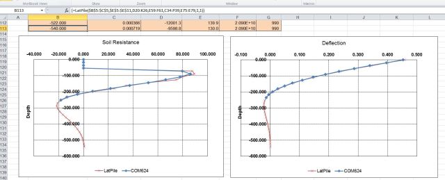
The final example is Example 4 from the COM624 manual, which uses 7 user input PY curves. In this case the COM624 program interpolates stiffness values between the curves above and below for each point down the pile, whereas the spreadsheet uses the values from the specified curve to apply to each layer. The spreadsheet input for this example is shown below:

Input for COM624 Example 4

In spite of the different method of application of the stiffness from the PY curves, the spreadsheet shows good agreement with the COM624 results:

Results for COM624 Manual Example 4

Results for COM624 Manual Example 4