Following the previous post I will now look in more detail at the functions in the py_Interpolate spreadsheet included in the download file:

py_SciPy.zip

Details of the required pyxll package (including download, free trial, and full documentation) can be found at: pyxll

For those installing a new copy of pyxll, a 10% discount on the first year’s fees is available using the coupon code “NEWTONEXCELBACH10”.

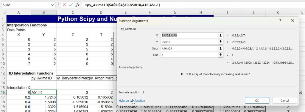
The py_Interpolate spreadsheet has 10 user defined functions linking to the Scipy spline interpolation functions. The Scipy help on each function is easily accessed from within Excel:

Open the “Insert Function” dialog, then click on “Help on this function” in the bottom left corner.

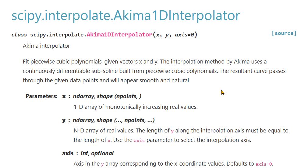
That takes you straight to the Scipy on-line help:

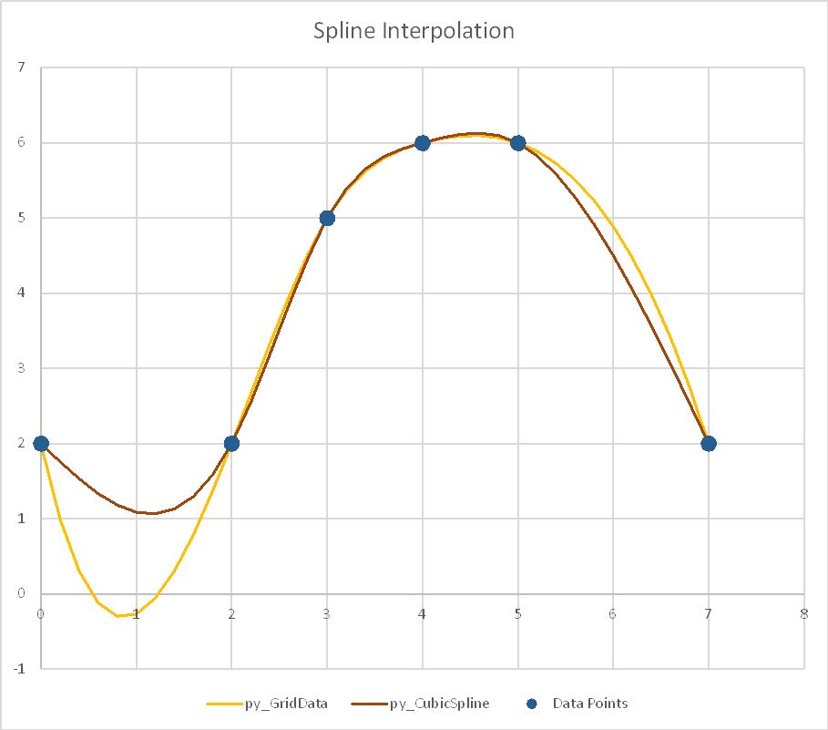
The examples in the spreadsheet plot the same data using each of the 9 functions. The screenshots below compare the output from the py_CubicSpline function, with “natural” end conditions, with the other nine functions:

py_Akima1D:

py_BarycentricInterp:

scipy.interpolate.barycentric_interpolate

scipy.interpolate.barycentric_interpolate(xi, yi, x, axis=0)

Convenience function for polynomial interpolation.

Constructs a polynomial that passes through a given set of points, then evaluates the polynomial. For reasons of numerical stability, this function does not compute the coefficients of the polynomial.

This function uses a “barycentric interpolation” method that treats the problem as a special case of rational function interpolation. This algorithm is quite stable, numerically, but even in a world of exact computation, unless the x coordinates are chosen very carefully – Chebyshev zeros (e.g., cos(i*pi/n)) are a good choice – polynomial interpolation itself is a very ill-conditioned process due to the Runge phenomenon.

py_KroghInterp:

scipy.interpolate.krogh_interpolate

scipy.interpolate.krogh_interpolate(xi, yi, x, der=0, axis=0)

Convenience function for polynomial interpolation.

See KroghInterpolator for more details.

py_GridData1

scipy.interpolate.griddata

scipy.interpolate.griddata(points, values, xi, method=’linear’, fill_value=nan, rescale=False)

Interpolate unstructured D-D data.

py_UniSpline

scipy.interpolate.UnivariateSpline

class scipy.interpolate.UnivariateSpline(x, y, w=None, bbox=[None, None], k=3, s=None, ext=0, check_finite=False)

1-D smoothing spline fit to a given set of data points.

Fits a spline y = spl(x) of degree k to the provided x, y data. s specifies the number of knots by specifying a smoothing condition.

py_Splev

scipy.interpolate.splev

scipy.interpolate.splev(x, tck, der=0, ext=0)

Evaluate a B-spline or its derivatives.

Given the knots and coefficients of a B-spline representation, evaluate the value of the smoothing polynomial and its derivatives. This is a wrapper around the FORTRAN routines splev and splder of FITPACK.

py_CubicSplineS

scipy.interpolate.CubicSpline

class scipy.interpolate.CubicSpline(x, y, axis=0, bc_type=’not-a-knot’, extrapolate=None)

Cubic spline data interpolator.

Interpolate data with a piecewise cubic polynomial which is twice continuously differentiable [1]. The result is represented as a PPoly instance with breakpoints matching the given data.

py_Interp1d(

scipy.interpolate.interp1d

class scipy.interpolate.interp1d(x, y, kind=’linear’, axis=-1, copy=True, bounds_error=None, fill_value=nan, assume_sorted=False)

Interpolate a 1-D function.

Legacy

This class is considered legacy and will no longer receive updates. This could also mean it will be removed in future SciPy versions.

py_Pchip

scipy.interpolate.PchipInterpolator

class scipy.interpolate.PchipInterpolator(x, y, axis=0, extrapolate=None)

PCHIP 1-D monotonic cubic interpolation.

x and y are arrays of values used to approximate some function f, with y = f(x). The interpolant uses monotonic cubic splines to find the value of new points. (PCHIP stands for Piecewise Cubic Hermite Interpolating Polynomial).