Solving polynomials – update

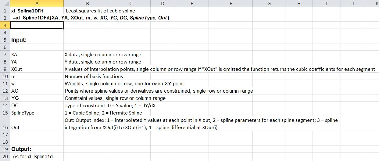
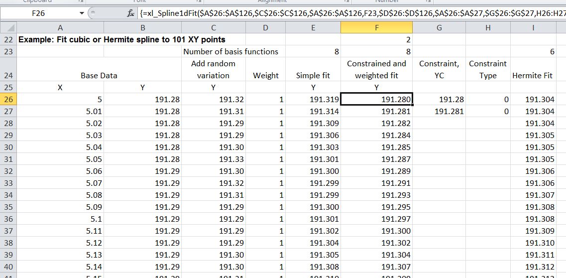
The polynomial spreadsheet (details here) provides functions to solve polynomial equations of any order; using an “exact” method for up to quartic, and an iterative procedure for higher orders.  The input for the functions requires the equation coefficients to be in a continuous column or row range.  This is convenient for many cases, but there are times when it is necessary to enter each coefficient separately.

I have now added a new function to the spreadsheet, which has the coefficients entered separately, and calls the appropriate solver function, depending on the number of coefficients.  The new function, including full open source code, may be downloaded from Polynomial.zip.The screenshot below shows an example of usage of the new function (included in the download file):

Polynomial1In this example three coefficients of a cubic equation are constant, but the fourth varies. The solution to the equation can be set up easily as follows:

  • Enter the values for coefficients a to c in any convenient range.
  • Enter the values for coefficient d in a column
  • In the cell adjacent to the top of the d column, enter the SolvePoly function:
    =solvepoly($B$12,$B$13,$B$14,C12).  Note the $ signs, making the first three addresses absolute (i.e. they will not change when the function is copied).
  • To display the three solutions and the number of real roots enter the function as an array function: select the function cell and the adjacent three cells; press F2; press ctrl-shift-enter.
  • These four cells may now be copied to the clipboard and pasted over as many rows as required.  Note that the first three coefficients always refer to the fixed range, but the d coefficient changes as it is copied down.
Posted in Arrays, Excel, Maths, UDFs, VBA | Tagged , , , , , | 1 Comment

Faster Biaxial Bending

The spreadsheet to calculate ultimate moment capacity of a reinforced or prestressed concrete section under combined axial load and biaxial bending, last presented here, has been updated to use the QuadBrent solver, rather than the Excel Goal Seek function, for better performance. The new solver function reduces the time to calculate the neutral axis angle from about 1 second down to 2 to 5 milliseconds, which is quite a respectable improvement in performance.

The new file can be downloaded from ULS Design Functions, including full open-source code.

The screenshot below shows the new FindNAAng function, which returns the calculated Neutral Axis angle for the specified combination of axial load and biaxial bending:

Biax-2-1

As in the previous version, the Neutral Axis angle may be entered manually on the input sheet, or updated automatically with the Adjust NA Angle button:
Biax-2-2

An output summary is given on the input sheet (as shown above) or detailed output data is provided on the Out sheet.  Alternatively interaction diagrams may be plotted for a range of neutral axis angles, as shown below:
Biax-2-3

See the previous post, or download, for more details.

Posted in Beam Bending, Concrete, Excel, Newton, UDFs, VBA | Tagged , , , , , , , , | 1 Comment

Alglib/Python spline functions update

The Excel Spline-Matrix spreadsheet has now been updated with several new spline interpolation functions.  See Alglib/Python linear and non-linear fitting functions for links to download and install the necessary Excel-Python and Alglib files.  Also required is Python version 2.7 or 2.6.

The spline functions included in the new version are:
xl_Spline3-01

Of which, the new ones are:

xl_PSpline: Parametric spline interpolation
xl_Spline3-02

The parametric spline function generates a smooth curve through a series of points, which need not be in order of increasing X.  Output may be specified to be periodic, in which case the curve is extended to the starting point, with slopes adjusted to provide a smooth curve throughout:
xl_Spline3-03

xl_Ratinterp provides rational interpolation without poles.  See the Alglib User Guide for background information.
xl_Spline3-04

xl_RatInterp output compared with a cubic spline
xl_Spline3-05

xl_Spline3D provides 3D Cubic spline interpolation.  The screenshot below shows a very simple example, taken from the Alglib manual.
xl_Spline3-06

xl_RBF and xl_RBFGrid provide Radial Basis Function interpolation.  Again see the Alglib User Guide for background information.
xl_Spline3-07

In this example the xl_RBF function is used to interpolate concrete shrinkage data, as used in the xl_NonLinFit example:
xl_Spline3-08

The xl_RBFGrid function provides the same results, but with more convenient data input, when 2D data is arranged in grid format.
xl_Spline3-09

Posted in AlgLib, Arrays, Excel, Link to Python, Maths, Newton, UDFs, VBA | Tagged , , , , , , , , , , | 2 Comments

The Deserter

The Deserter is a traditional song featured on Fairport Convention’s 1968 album Liege and Lief; it is said to be the favourite track on the album of Sandy Denny, and the producer, Joe Boyd.  The song has a long history, and many versions.  Dave Swarbrick commented:

Although we learned this song from a faded Victorian broadside, it is much older in origin. It was the habit of broadside printers to bring older songs up to date—in this case by including the name of Prince Albert.

A detailed list of performances can be found at Mainly Norfolk.  It seems from some of the comments that some performers totally missed the irony in the closing verse.

Searching on “Ratcliff Highway” led me to this beautiful instrumental version:

and a live recording of a totally different traditional song, by The Dubliners:

Posted in Bach | Tagged , , , , | Leave a comment

Alglib/Python spline functions

Continuing from the previous post, the new xl_Spline-Matrix.zip spreadsheet includes functions for 1D and 2D linear and cubic splines.

xl_Spline2-1The basic 1D spline allows  for output of linear splines, or 5 different types of cubic spline, as listed above.

Output may be spline values at listed points, spline parameters for each spline segment, or spline integration or slope.

xl_Spline2-2
Additional data allows input of end slopes or curvatures for cubic splines, slope data for hermite splines, or end type and tension for Catmull-Rom splines:
xl_Spline2-3

The screenshots below show input and results for all six spline types, passing through 5 points:
xl_Spline2-4

xl_Spline2-5

Output of spline segment data, integration, and slope and curvature values is shown below:
xl_Spline2-6

Input and output for the 2D spline function is shown below.
xl_Spline2-7

The screenshots below show 2D splines fitted to tabular data for air density under varying pressure and temperature:
xl_Spline2-8

xl_Spline2-9

The xl_Spline1DFit function finds the least squares fit of a cubic spline with a specified number of segments, with optional weighting and/or constraints:
xl_Spline2-10

Alternative spline fits:
xl_Spline2-11

xl_Spline2-12

The xl_SplineInt and xl_SplineDiff functions provide integration and differentiation data for any of the spline types. They are equivalent to output options 3 or 4 with the xl_Spline1d function:
xl_Spline2-13

xl_Spline2-14

Posted in AlgLib, Excel, Link to Python, Maths, Newton, Numerical integration, UDFs, VBA | Tagged , , , , , , , , , , , | 1 Comment