Previous Python Post
The basic range of data types in Python is quite simple, but by the time we have added additional types used in the numpy package, and translation of Excel data types into the Python equivalent the picture gets considerably more complicated, and you can find yourself wasting significant amounts of time chasing down errors due to using incompatible data types. This post will look at the main data types, including numpy arrays, with examples of their use in PyXll functions.
The Python code and associated Excel spreadsheet can be downloaded from pyTypes.zip. To use the Python functions it is necessary to install the PyXll add-in, then either add “pyTypes” under modules in the pyxll.cfg file, or simply copy and paste all the code from pyTypes.py into the worksheetfuncs.py file, to be found in the PyXll\examples folder.
The PyXll manual lists the following PyXll data types, with their Python equivalent:

PyXll and Python Data Types
Note that the unicode type is only available from Excel 2007.
An Excel range of any of the above data types can be passed as a 2D array, which is treated in Python as a “list of lists”. In addition the PyXll var type can be used for any of the above types, or a range. A further option for transferring an Excel range of numerical data is use of the numpy_array, numpy_row and numpy_column types. Further options (which we will examine in a later post) are Custom Types and the xl_cell type.
The function var_pyxll_function_1 shown below (taken from the PyXll worksheetfuncs.py file) returns the name of the data type passed to the function. The var_pyxll_function_1a function simply returns the data back to the spreadsheet.
@xl_func("var x: string")
def var_pyxll_function_1(x):
    """takes an float, bool, string, None or array"""
    # we'll return the type of the object passed to us, pyxll
    # will then convert that to a string when it's returned to
    # excel.
    return type(x)

@xl_func("var x: var")
def var_pyxll_function_1a(x):
    return x
Examples of these functions are shown in the screenshot below:
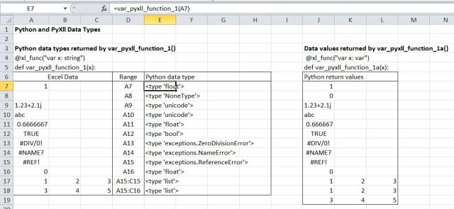
Python basic data types
The var_pyxll_function_1 function passes data to Python as a var, and returns a string with the Python data type name. Note that:
- All numbers (including integers) become Python floats.
- Empty cells become Python NoneType
- Strings (including complex number strings) become Python Unicode (in Excel 2007 and later).
- Boolean values become Python bool.
- Excel error values become different types of Python exceptions.
- Both 1D and 2D Excel ranges become Python lists. In fact in both cases the range becomes a “list of lists”.
The var_pyxll_function_1a function passes data to Python as a var, and simply returns the same data, without modification:
- All data types other than a blank, including 1D and 2D ranges and error values, are passed back unchanged, however blank cells are passed back as a zero.
Further details of the handling of data are examined in four variants of a function converting an Excel complex number string to a pair of floating point values in adjacent cells:
@xl_func("var x: var")
def py_Complex1(x):
    """
    Convert a complex number string to a pair of floats.
    x:  Complex number string or float.
    """
    if isinstance(x, float) == False:
        if x[-1] == "i":
            x = x.replace("i", "j",1)
    c = complex(x)
    clist = list([[0.,0.]])
    clist[0][0] = c.real
    clist[0][1] = c.imag
    return clist
The code first checks if the function argument is a float. If not it checks if the last character is an “i” (the default Excel imaginary number indicator), and if so changes it to a “j” (the required character for a Python complex number). The code then:
- Converts the Excel complex number string to a Python complex number.
- Creates a python “list of lists” consisting of a single list containing two floats: [0., 0.]
- Allocates the real and imaginary parts of the complex number to the list. Note that the index values are always base zero, and that two index values are required; the first indicating list index 0 (i.e. the first and only list in the list of lists) and the second indicating the index value in the selected list.
- The resulting list is then returned with the statement: return clist
Note the use of text within triple quotes at the top of the function. This text will appear in the “Excel function wizard”, including the description of each function argument. This feature will be examined in more detail in a later post.
The results of this function are shown below:
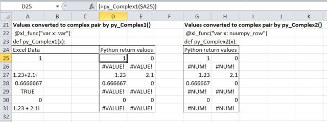
Results from py_Complex1 and py_Complex2
Note that the complex number string in cell A27 is returned as a pair of values, and the other cells with numerical values are correctly returned with the cell value as the real part, and an imaginary value of zero. The blank and Boolean values return a #VALUE! error, as does the string in cell A31, because it has spaces around the “+”, which are not allowed in a complex number string.
The function py_Complex2 is similar, except that the return type has been changed from a var to a numpy_row:
@xl_func("var x: numpy_row")
def py_Complex2(x):
    """
    Convert a complex number string to a pair of floats.
    x:  Complex number string or float.
    """
    crow = zeros(2)
    if isinstance(x, float) == False:
        if x[-1] == "i":
            x = x.replace("i", "j",1)
    c = complex(x)
    crow[0] = c.real
    crow[1] = c.imag
    return crow
A numpy_row is a 1D array created with the statement: crow = zeros(x), where x is the number of elements in the array. Since it is a 1D array each element is specified with a single index, e.g. crow[0] = c.real.
The results for py_Complex2 are the same as py_Complex1, except that invalid input returns a #NUM! error, rather than #VALUE!
In py_Complex3 a check has been added to pick up invalid input data, so a more useful error message can be returned:
@xl_func("var x: var")
def py_Complex3(x):
    """
    Convert a complex number string to a pair of floats.
    x:  Complex number string or float.
    """
    try:
        crow = zeros(2)
        if isinstance(x, float) == False:
            if x[-1] == "i":
                x = x.replace("i", "j",1)
        c = complex(x)
        crow[0] = c.real
        crow[1] = c.imag
        return array([crow])
    except:
        return "Invalid input type"
In this case the return array has been created as a 1D numpy-row, using crow = zeros(2), but the return value may also be the string “Invalid input type”. To handle these alternative data types the return value must be specified as a var, and the numpy_row is converted into a 2D array with: return array([crow]).
Note the use of the Python “try:, except:” keywords to handle the exception raised when the statement: c = complex(x) is applied to an x that is not a valid complex number string or a float.
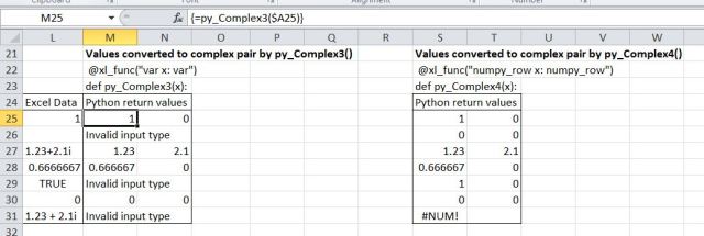
py_Complex3 and py_Complex4
In py_Complex4 the check of the input data type has been amended to first check for a float or a Boolean (in which case the value is returned), then check for a string. A blank cell does not satisfy any of these conditions, and returns a value of zero. The numpy_row return type has been used, which precludes returning a string, but this could be changed to a var, as in py_Complex3, to allow an error message to be returned for invalid string input.
@xl_func("var x: numpy_row")
def py_Complex4(x):
    """
    Convert a complex number string to a pair of floats.
    x:  Complex number string or float.
    """
    crow = zeros(2)
    if isinstance(x, float) or isinstance(x, bool):
        crow[0] = x
    elif isinstance(x, unicode):
        if x[-1] == "i":
            x = x.replace("i", "j",1)
        c = complex(x)
        crow[0] = c.real
        crow[1] = c.imag
    else:
        crow[0] = 0
    return crow
The use of different types of array is illustrated with three variants of a function to sum the values in each row of a 2D range, and return the results as a column array.
@xl_func("float[] x: float[]")
def SumRows1(x):
    """
    Sum rows of selected range.
    x:  Range to sum.
    """
    nrows = len(x)
    i = 0
    suml = [0.] * nrows
    for row in x:
       for j in range(0,3):
            suml[i] = suml[i] + row[j]
       i = i+1
    return transpose([suml])

@xl_func("var x: var")
def SumRows2(x):
    """
    Sum rows of selected range.
    x:  Range to sum.
    """
    nrows = len(x)
    i = 0
    suml = [0.] * nrows
    for row in x:
       for j in range(0,3):
            suml[i] = suml[i] + row[j]
       i = i+1
    return transpose([suml])

@xl_func("numpy_array x: numpy_column")
def SumRows3(x):
    """
    Sum rows of selected range.
    x:  Range to sum.
    """
    nrows = len(x)
    i = 0
    suml = zeros(nrows)
    for row in x:
       for col in row:
            suml[i] = suml[i] + col
       i = i+1
    return suml
This code uses two variants of a for loop:
- for row in x: loops three times to return a list of 3 values for each of the three rows in x
- for j in range(0, 3): loops three times returning the values 0, 1, 2
- the j value is then used as the index in row[j] to return each value in each row
The row sum values are assigned to the list suml, which is finally returned as a 2D array with 3 rows and 1 column with the line: return transpose([suml])
SumRows1 and SumRows2 are similar, except that SumRows2 uses vars for both input and output rather than float arrays (float[]).
In SumRows3 the input is a numpy_array, and output a numpy_column. suml is created as a 1D numpy array, using the zeros function, and because the return type has been declared as a numpy_column this can be returned without transposing.
The screenshot below shows that when the input array has numbers in every cell them the three functions produce identical results:
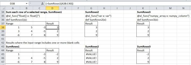
SumRows functions
However if one more cells are blank SumRows2 returns an error, whreas SumRows1 and SumRows2 allocate a zero to the blank cell, and return the correct results.
Finally the convenience of use of the numpy routines is illustrated with a function to solve systems of linear equations with a single line of Python code:
@xl_func("numpy_array a, numpy_column x: numpy_column")
def py_solve(a, x):
	"""
        Solve a matrix equation ax = y.
	a: square matrix
	x: column x vector
	"""
	return solve(a, x)
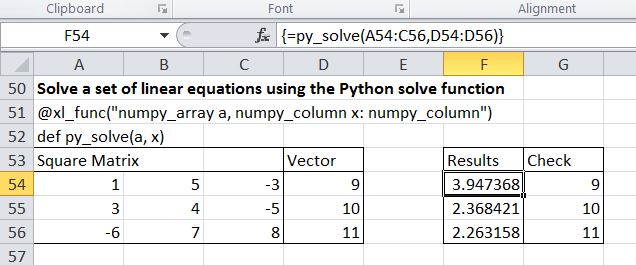
py_solve


