Linking Excel to Fortran, via xlwings, Python and ctypes

Continuing the recent series on using Fortran code published in Programming the Finite Element Method (5th ed. John Wiley & Sons, I.M. Smith, D.V. Griffiths and L. Margetts (2014)), this post looks at linking Excel to Fortran code compiled as a dll (dynamic link library).

It is quite possible to link Excel VBA directly to Fortran based dlls, but because Python provides a convenient link to numerous scientific and maths routines in Numpy, Scipy, and other libraries, I have chosen to create the link through Python, using xlwings.  The spreadsheet, dll files, and Python and Fortran code can be downloaded from:

PlateMC-dll.zip

To run the code requires Python and xlwings to be installed.  The Anaconda Python package includes xlwings by default, and also allows The MinGW package to be installed, which includes Gfortran.  GFortran is not required to run the application, but it is needed if you want to make any changes to the Fortran code and recompile.  The dll file may be copied to the same directory as the spreadsheet and Python file (Py64f.py), or to any directory on the system search path.

As for compiling an exe file and linking to Excel, the process is not difficult, but it is not well documented, and any deviation from the exact procedure is likely to result in errors accompanied with a collection of exceedingly unhelpful error messages.

In the previous version of this spreadsheet the data for the compiled program was written to the hard disk as text files, which were opened and read by the Fortran program, which then wrote back the results to the hard disk, to be opened and read by Excel.  This is a slow and cumbersome procedure, but it does remove all problems of differing data formats.  In contrast, when the data is transferred directly from Excel to the Fortran based dll it is essential all data and objects are in a format that is recognisable to both programs.  The procedure I have used to ensure data compatibility was:

  • In Excel VBA collect the input data as a series of named worksheet ranges, converted to variant arrays.
  • Transfer to Python with an xlwings UDF (user defined function).  Arrays are transferred as Python tuples.
  • Convert the tuples to Numpy arrays of the appropriate data type, and if necessary convert values to the correct data type.  For this application all values were either double64 or int (equivalent to VBA double and long).
  • Convert the arrays and values to c_type format, which is compatible with both C and Fortran.
  • Call the required function from the dll, passing all arguments by reference.
  • Return the result arrays and values to VBA using the original Python variables.
  • Paste the results to named ranges in the spreadsheet.
  • Update the deformed mesh plot in VBA.

The VBA code is straightforward.  The Sub P64py reads data from the ranges “Plate_def”, “Tolerance”, “srf”, and “props”, adjusting the range sizes where necessary, then calls the function xl_P64, which converts empty cells in the Plate_Def range to zeros, then calls the Python function py64 in the module Py64f.py.

The main features of the Python code are:

  • Import numpy, os and xlwings.
  • Import the required data types and methods from the ctypes library (byref, cdll, c_int, c_double), and import numpy.ctypeslib to handle Numpy arrays.
  • Load the dll file, using cdll.LoadLibrary (see Python code below).  The code is set up to look for the dll first in the workbook directory, or if that fails look anywhere on the search path.
  • The data from the “Plate_def” worksheet range is passed from VBA as a variant array with all numerical values passed as doubles.  In both Numpy and Fortran arrays must have a single data type, and the Fortran code requires some of the input data as doubles and some as integers.  For this reason the dataa array must be split into two separate arrays, containing doubles (meshdims) and integers (meshnums).
  • Arrays for the output data must be sized and created in Python, and passed as ctype pointers to Fortran, together with the size of any variable dimensions.
  • Having converted and created the required arrays in Numpy format, ctype pointers are created with statements such as:
    coordp = npc.as_ctypes(coorda)
    Note that it is important that the pointer has a different name to the Numpy array.
  • Values are converted to ctypes using c_int or c_double, e.g:
    nsrf = c_int(nsrfi)
  • The p64 function is called from p64dll, with all arguments passed “byref” (see code below)
  • The data passed to the Fortran code consists of pointers to the Python variables, hence the arrays and values returned from p64 may be accessed using the original Python variables names.

The full Python code is shown below:

import numpy  as np
from ctypes import byref, cdll, c_int, c_double, c_char_p
import numpy.ctypeslib as npc
import os
import time
import xlwings as xw

#Load p64s.dll
try:
    wkbpath = os.path.dirname(os.path.abspath(__file__))
    p64dll = cdll.LoadLibrary(wkbpath + '/p64s.dll')
except:
    p64dll = cdll.LoadLibrary('./p64s.dll')
    
def py64(dataa, tola, srfa, propa):
# Convert dataa to Numpy array, and split into double and integer arrays
    dataa = np.array(dataa)
    meshdims = dataa[0:2,:]
    meshnums = dataa[2:4,0:2].astype(int)

#Calculate size of output arrays    
    np_types = int(dataa[4,0])
    nx1 = meshnums[0,0]
    nx2 = meshnums[0,1]
    ny1 = meshnums[1,0]
    ny2 = meshnums[1,1]
    nye=ny1+ny2
    nels=nx1*nye+ny2*nx2
    nn=(3*nye+2)*nx1+2*nye+1+(3*ny2+2)*nx2
#Create Numpy arrays and convert to ctypes pointers
#Convert integers to c_int
    coorda = np.zeros((nn,2))
    coordp = npc.as_ctypes(coorda)
    g_num = np.zeros((nels,8), dtype=np.int)
    g_nump = npc.as_ctypes(g_num)
    srfa = np.array(srfa)[:,0]
    nsrfi = srfa.shape[0]
    nsrf = c_int(nsrfi)
    nodedisa = np.zeros((nn,nsrfi*3))
    nodedisp = npc.as_ctypes(nodedisa)
    nnp = c_int(nn)
    meshdimp = npc.as_ctypes(meshdims)
    meshnump = npc.as_ctypes(meshnums)
    tolp = npc.as_ctypes(np.array(tola)[0])
    srfp = npc.as_ctypes(srfa)
    propa = np.array(propa)
    propp = npc.as_ctypes(propa)
    resa = np.zeros((5,nsrfi))
    resp = npc.as_ctypes(resa)
    np_types = c_int(np_types)
    nelsp = c_int(nels)
    
 #Call p64 with all ctype arguments passed by reference   
    iErr = p64dll.p64(byref(resp), byref(meshdimp), byref(meshnump), byref(tolp), byref(srfp), byref(nsrf), 
    byref(propp), byref(np_types), byref(coordp), byref(nnp), byref(nodedisp), byref(g_nump), byref(nelsp))
 
 #Return results using original Python variables
    return [resa, coorda, nodedisa, g_num, nn,  nels] 

The Fortran code requires an interface to read input data and return results. Note that dynamic arrays must have their size defined by integer arguments passed from the calling program. Also note that Fortran arrays are defined in the opposite direction to Python and VBA arrays (i.e. columns, rows):

module main
implicit none
integer, parameter:: dp=SELECTED_REAL_KIND(15)

contains

...  Functions called by p64

END module main

integer function p64(resa, meshdims, meshnums, tola, srfa, nsrf, prop, &
   np_types, g_coord, nn, NodeDisp,g_num, nels)
!-------------------------------------------------------------------------
! Program 6.4 Plane strain slope stability analysis of an elastic-plastic
!             (Mohr-Coulomb) material using 8-node rectangular
!             quadrilaterals. Viscoplastic strain method.
!-------------------------------------------------------------------------
  use main
  implicit none 
 integer, intent(in):: meshnums(2,2), nsrf, np_types, nn, nels
 integer, intent(out):: g_num(8,nels)
 real(dp),INTENT(IN)::meshdims(3,2), tola(3), srfa(nsrf), prop(7,np_types)
 real(dp),INTENT(OUT)::resa(nsrf,5), g_coord(2,nn), NodeDisp(nsrf*3,nn)

...
  

The Fortran code is compiled to a dll as shown below:

  • gfortran -shared -fno-underscoring -o p64.dll P64dll.f03

As for the compilation of an exe file, if the program is to run on a computer without MinGW it must be compiled with the -static option:

  • gfortran -shared -static -fno-underscoring -o p64s.dll P64dll.f03


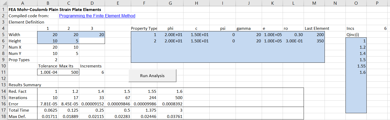
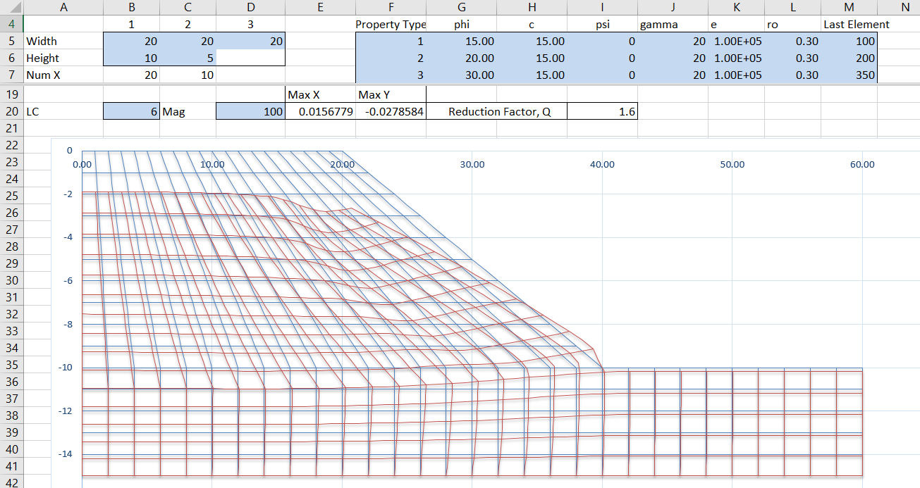
The resulting output is shown below:

PlaneStrain5-1

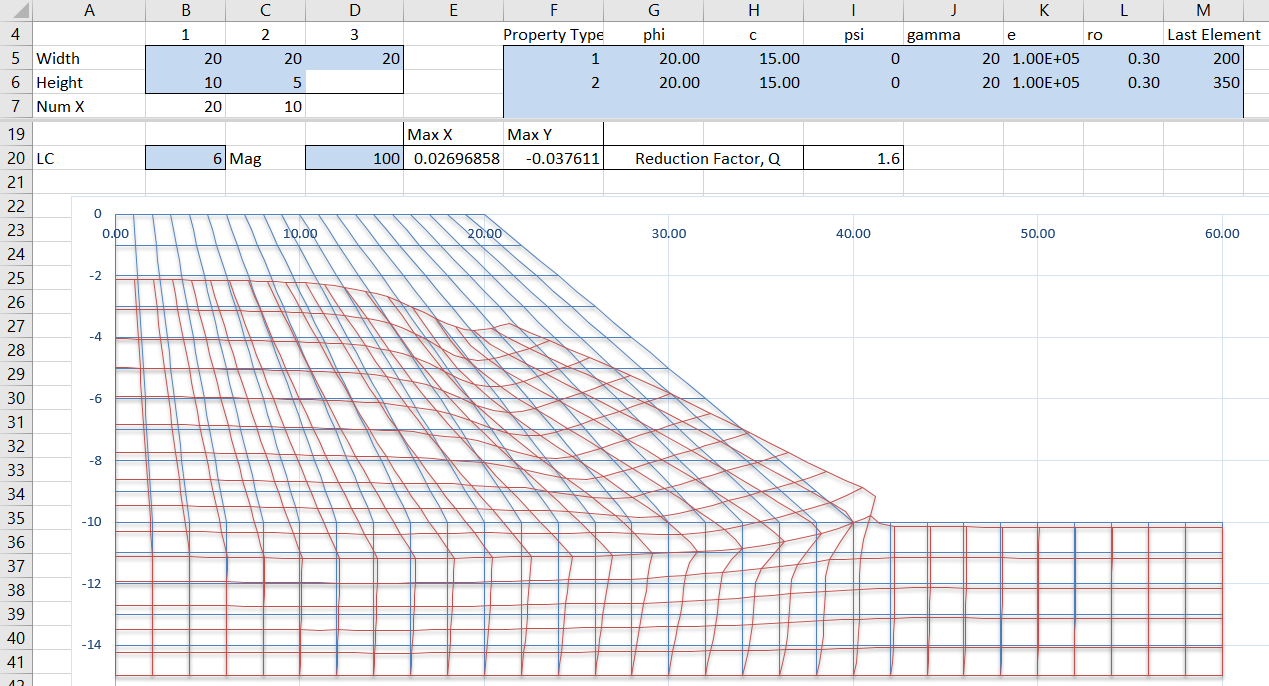
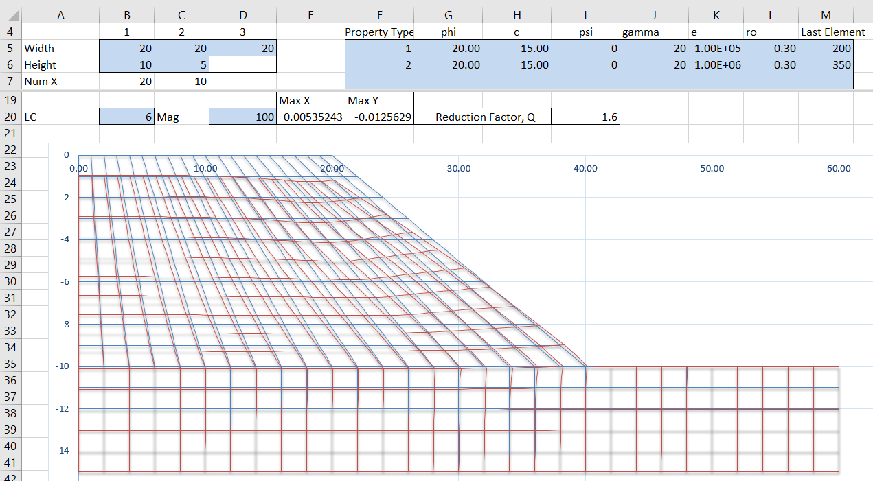
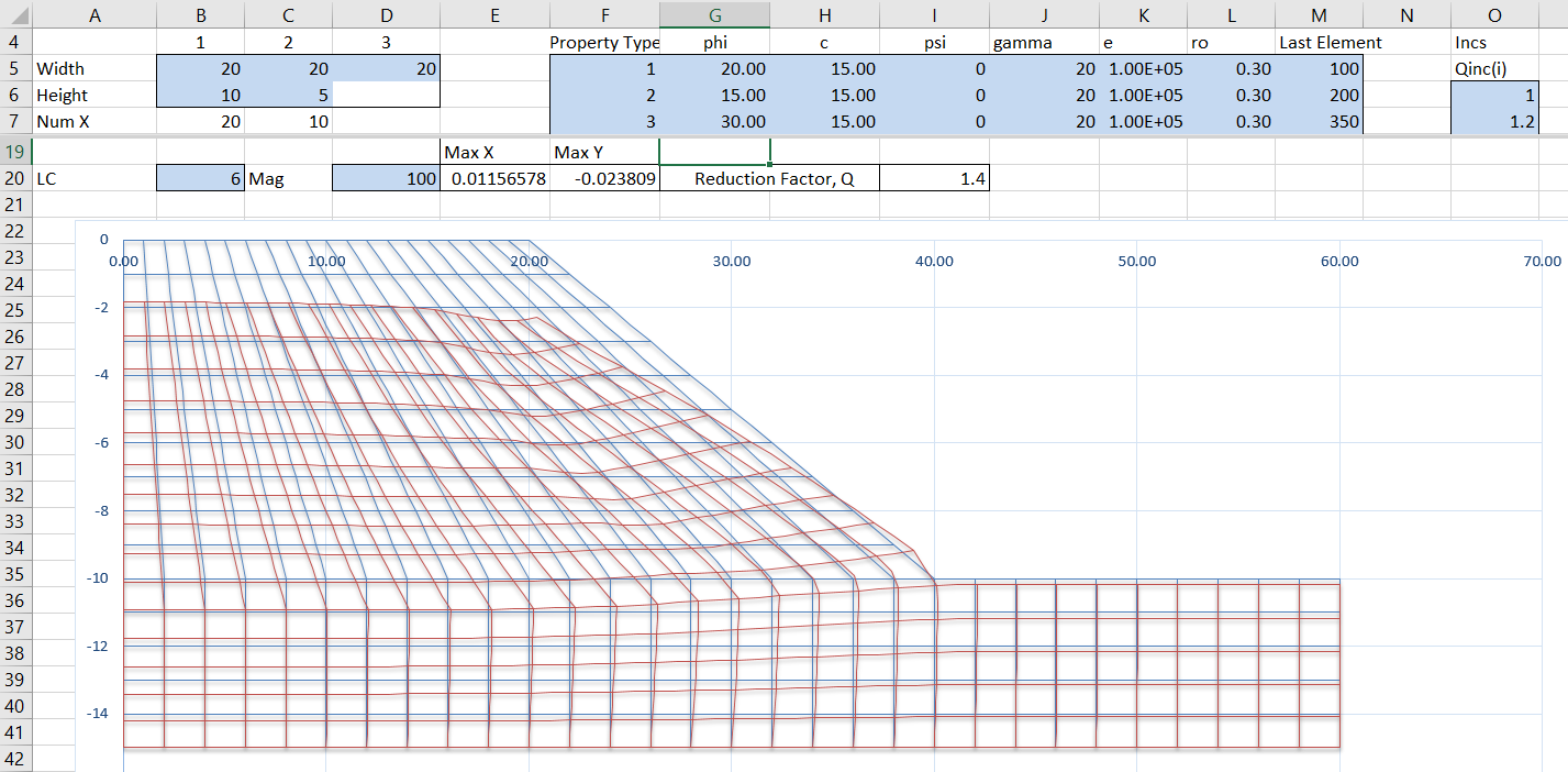
The VBA plotting routine has been re-written to allow changes in the number of elements to be plotted.

PlaneStrain5-2

PlaneStrain5-3

See the next post for further examples and discussion of results with varying element size.

Posted in Excel, Finite Element Analysis, Fortran, Geotechnical Engineering, Link to dll, Link to Python, Newton, NumPy and SciPy, VBA | Tagged , , , , , , , , , , | 2 Comments

Compiling Fortran code for Windows

This post is a continuation of a recent series, using Fortran code published in  Programming the Finite Element Method (5th ed. John Wiley & Sons, I.M. Smith, D.V. Griffiths and L. Margetts (2014)).

The compiled file provided in the download should run on any Windows computer, but to edit the code in any way, recompilation is required.  The process is not difficult, but it is not well documented, at least for those not familiar with Fortran, so this post will provide a detailed description of the process, and some alternative options.

For this exercise I have used the MinGW package (Minimalist GNU for Windows), which includes the GFortran compiler.  MinGW may be installed from the Anaconda Python package.  It is not included in a default install of Anaconda, but it may be easily added with the command: conda install mingw.

Alternatively installation instructions for just MinGW are provided here.

The Fortran code to be compiled consists of the main program and 17 sub-routines.  To keep the compilation process as simple as possible the sub-routines can be included in the same text file as the main program.  The code using this approach in the original download included a block of  “interface” statements:

INTERFACE
!
SUBROUTINE getname(argv,nlen)
IMPLICIT NONE
INTEGER::narg
INTEGER,INTENT(OUT)::nlen
CHARACTER(*),INTENT(OUT)::argv
INTEGER::lnblnk,iargc
END SUBROUTINE getname
!
SUBROUTINE emb_2d_bc(nx1,nx2,ny1,ny2,nf)
IMPLICIT NONE
INTEGER,INTENT(IN)::nx1,nx2,ny1,ny2
INTEGER,INTENT(OUT)::nf(:,:)
END SUBROUTINE emb_2d_bc
...
15 more subroutines
...
END SUBROUTINE
END INTERFACE

This is not necessary however. The revised code is shown in outline below, and is included in full in the download file:

PROGRAM p64
!-------------------------------------------------------------------------
! Program 6.4 Plane strain slope stability analysis of an elastic-plastic
!             (Mohr-Coulomb) material using 8-node rectangular
!             quadrilaterals. Viscoplastic strain method.
!-------------------------------------------------------------------------
 IMPLICIT NONE
 !
 INTEGER,PARAMETER::iwp=SELECTED_REAL_KIND(15)
 INTEGER::i,iel,iters,iy,limit,ndim=2,ndof=16,nels,neq,nip=4,nlen,nn,     &
 ! ... Main Program
 ! ...
    END DO
!
!   IF(iters==limit)EXIT
END DO srf_trials
RETURN
!
contains
! 17 subroutines:
SUBROUTINE getname(argv,nlen)
!
! This subroutine reads the base name of data file.
!
 IMPLICIT NONE
 …
CASE DEFAULT
   WRITE(*,*)"nst size not recognised in formm"
 END SELECT
RETURN   
END SUBROUTINE formm
END PROGRAM p64

This code, in P64-1.f03, is compiled by opening a command window and entering:

PlaneStrain4-1

This generates the file P64.exe, which can be called from PlateMC-exe.xlsb, as described in the previous posts.  Note that the exe file created requires MinGW to be installed.  See below for the compilation option to generate a stand-alone file.

As a step towards separating out the subroutines into a library of general purpose routines, the subroutines can be defined as a separate module, within the same file:

PROGRAM p64
!-------------------------------------------------------------------------
! Program 6.4 Plane strain slope stability analysis of an elastic-plastic
!             (Mohr-Coulomb) material using 8-node rectangular
!             quadrilaterals. Viscoplastic strain method.
!-------------------------------------------------------------------------
 USE main 
!
 IMPLICIT NONE
 !
 INTEGER,PARAMETER::iwp=SELECTED_REAL_KIND(15)
 …
    END DO
!
!   IF(iters==limit)EXIT
END DO srf_trials
RETURN
END PROGRAM p64
!
module main
contains
SUBROUTINE getname(argv,nlen)
!
! This subroutine reads the base name of data file.
!
 IMPLICIT NONE
 …
 CASE DEFAULT
   WRITE(*,*)"nst size not recognised in formm"
 END SELECT
RETURN   
END SUBROUTINE formm
end module main

Note the changes:

  • Addition of the USE MAIN statement
  • The END PROGRAM P64 is moved to the end of the top level code
  • The statement MODULE MAIN is added at the top of the subroutine code, and END MODULE MAIN at the end.

This code, saved as P64-2.f03, is compiled in the same format as before.

The next stage is to extract all the code from MODULE MAIN to END MODULE MAIN into a separate file, named main.f03.  This is then compiled in two stages as shown below:

PlaneStrain4-2

The command: gfortran -c main.f03 creates the file main.o, which is then compiled with p64-3.f03 to create P64.exe.

The final stage is to compile to a stand alone executable file, with the “-static” statement:

PlaneStrain4-3

The download file includes all the code files described above, as well as the stand alone executable file, the spreadsheet, and example results files.

Posted in Excel, Finite Element Analysis, Fortran, Newton, VBA | Tagged , , , , , , , | 2 Comments

Running exe files from Excel

Following on from the previous post (running a compiled Fortran finite element analysis program from Excel), this post looks at the details of calling any command line routine from Excel, through VBA.  The important points that need to be addressed are:

  • Writing any required data files
  • Calling the program from the required directory, including any required arguments
  • Ensuring that the VBA code waits until the external routine has finished before proceeding.
  • Reading the output files, and transferring the required data to Excel, in the correct format

The PlateMC-exe spreadsheet uses the code below to write the data file:

Sub P64exe()
Dim P64Dat As Variant, FName As String, DatPath As String, i As Long, ExeFile As String, Res As Variant
Dim iErr As Variant, STime As Double, ResA() As Double, NumRows As Long, j As Long, Numcols As Long, k As Long, Off As Long
Dim DataA  As Variant, TolA As Variant, PropA As Variant, Nsrf As Long, SRFA As Variant, np_types As Long, Row As Long
Dim wsh As Object, waitOnReturn As Boolean, windowStyle As Integer

Const NProps As Long = 7, ExeName As String = "P64"
    STime = Timer

' Read data
    DataA = Range("Plate_Def").Value2
    TolA = Range("tolerance").Value2
    Nsrf = Int(TolA(1, 3))
    Range("srf").Resize(Nsrf, 2).Name = "srf"
    SRFA = Range("srf").Value2
    np_types = DataA(5, 1)

    Range("props").Resize(np_types, NProps).Name = "props"
    PropA = Range("props").Value2
    Numcols = NProps
    If Nsrf > NProps Then Numcols = Nsrf

    ReDim P64Dat(1 To 6 + np_types, 1 To Numcols)

    For i = 1 To 3
        P64Dat(1, i) = DataA(1, i)
    Next i
    For i = 4 To 5
        P64Dat(1, i) = DataA(2, i - 3)
    Next i
    P64Dat(2, 1) = DataA(3, 1)
    P64Dat(2, 2) = DataA(3, 2)
    P64Dat(2, 3) = DataA(4, 1)
    P64Dat(2, 4) = DataA(4, 2)
    P64Dat(3, 1) = DataA(5, 1)
    For i = 1 To np_types
        For j = 1 To NProps
            P64Dat(i + 3, j) = PropA(i, j)
        Next j
    Next i
    P64Dat(i + 3, 1) = TolA(1, 1)
    P64Dat(i + 3, 2) = TolA(1, 2)
    P64Dat(i + 4, 1) = Nsrf

    For j = 1 To Nsrf
    P64Dat(i + 5, j) = SRFA(j, 1)
    Next j

Note that:

  • Data is read from four separate named ranges on the spreadsheet
  • It is transferred to an array (P64Dat), with the data arranged in the format required by the external program (P64.exe)
  • The array is then written to a text file (P64.Dat), in the same directory as the spreadsheet, with the code shown below (the commented out line shows an alternative of reading the required directory from a named worksheet range)
' Write data to text file
    DatPath = ThisWorkbook.Path & "\"
    ' DatPath = Range("datpath").Value2
    FName = DatPath & "P64.dat"
    iErr = PrinttoFile(P64Dat, FName)

The PrinttoFile function:

Function PrinttoFile(Dat As Variant, FileName As String)
Dim FNum As Long, TxtLine As String, i As Long, Row As Long, Numcols As Long

    If TypeName(Dat) = "Range" Then Dat = Dat.Value2
    Numcols = UBound(Dat, 2)
    On Error GoTo rtnerr
    FNum = FreeFile
    Open FileName For Output Access Write As FNum

    For Row = 1 To UBound(Dat)
        TxtLine = ""
        For i = 1 To Numcols
            If IsEmpty(Dat(Row, i)) = False Then
                TxtLine = TxtLine & Dat(Row, i) & "  "
            End If
        Next i
        Print #FNum, TxtLine
    Next Row
    Close FNum
    PrinttoFile = 0
    Exit Function
rtnerr:
    Close FNum
    PrinttoFile = Err.Description
End Function

P64.exe can then be called using the WScript.Shell object:

' Run P64.exe
    Set wsh = VBA.CreateObject("WScript.Shell")
    waitOnReturn = True
    windowStyle = 1
    ExeFile = "cmd /C  CD " & DatPath & "& " & ExeName & " p64"
    iErr = wsh.Run(ExeFile, windowStyle, waitOnReturn)

    If iErr <> 0 Then GoTo rtnerr

More details of the windowStyle options can be found at Shell Function

Information on using the scripting shell object is strangely scattered, but the format shown above succeeds in changing directory to the location specified in DatPath, then running the program with the argument p64.  Note that the variable ExeFile resolves to:

  • cmd /C  CD  DatPath &  ExeName  p64

The “&” in the command line is required to combine the CD (change directory) command with the command to run the program named by ExeName.

With windowStyle set to 1 the program runs in a cmd window, as shown below:

PlaneStrain3-1

When the external program is complete the command window closes and control returns to the VBA code, which can then read the results files, and return the required results to the spreadsheet:

' Read result files
    FName = DatPath & "P64.res"
    Res = ReadText(FName)
    Res = SplitText(Res, 5, , , , True)
    Range("res").ClearContents
    Range("res").Resize(5, UBound(Res)).Name = "res"
    Range("Res").Value2 = TranspV(Res)
    FName = DatPath & "P64.rs2"
    Res = ReadText(FName)
    Res = SplitText(Res, 3, , , , True)
    NumRows = UBound(Res) / Nsrf
    Numcols = Nsrf * 3
    ReDim ResA(1 To NumRows, 1 To Numcols)
    On Error Resume Next
    Off = 0
    Row = 2
    For i = 1 To Nsrf
        For j = 1 To NumRows
            For k = 1 To 3
                ResA(j, k + Off) = Res(Row, k)
            Next k
            Row = Row + 1
        Next j
        Off = Off + 3
    Next i
    Range("def").Resize(NumRows, Numcols).Name = "def"
    Range("def").Value2 = ResA

    FName = DatPath & "P64.msh"
    Res = ReadText(FName)
    Res = SplitText(Res, 2, , , , True)
    ReDim ResA(1 To UBound(Res), 1 To 2)
    For i = 1 To UBound(Res)
        ResA(i, 1) = CDbl(Res(i, 1))
        ResA(i, 2) = CDbl(Res(i, 2))
    Next i
    Range("g_coord").Resize(UBound(Res), 2).Name = "g_coord"
    Range("g_coord").Value2 = ResA

    Exit Sub
rtnerr:

    End Sub
Posted in Computing - general, Excel, Finite Element Analysis, Fortran, Geotechnical Engineering, Newton, VBA | Tagged , , , , , , , | 2 Comments

Making non-linear FEA with Excel go (much) faster

The spreadsheet presented in the previous post takes about 90 seconds to complete (with the iteration limit set at 500) on my computer, and is much slower on some other systems.  The VBA code that does all the hard work is based on Fortran code published in  Programming the Finite Element Method, 5th ed. John Wiley & Sons, I.M. Smith, D.V. Griffiths and L. Margetts (2014), so I have now linked the spreadsheet input to a modified version of the compiled Fortran code.

Download PlateMC-exe.zip, including full open source code.

To run the program, copy all the contents of the zip file to the same directory, and it should work.

As can be seen in the screen shot below (click on any image for a full-size view), changing to compiled code has resulted in a huge improvement in run time, reducing the total time to 3 seconds, a factor of 30.

PlaneStrain2-1

At this stage I have compiled the Fortran code as an exe file, that reads the input data from a text file (generated by Excel), and writes the results to 3 results text files, which are then read and parsed in VBA.  This is not the most efficient way to transfer data to and from compiled programs, but it is the easiest to implement, and the overall effect on the run time is totally negligible.

The next post in this series will look at the VBA code required to generate the input data file, run the exe file, and read the results, and will be followed by the procedure for compiling the Fortran code, using the open source MinGW and GFortran programs.

The spreadsheet input is the same as the previous version, except that elements allocated with each soil property type are now specified in the property table.  The elements are numbered from left to right, and top to bottom, so the input in the screen shot below shows Property Type 1 allocated to the first 200 elements, forming the soil slope, and Property Type 2 to the remaining 150 elements in the foundation layers.  In this example both of the material types have been allocated the same properties, which are the same as in the previous post.  The number of iterations and element deflections are almost identical to those from the VBA code.  The reported residual error and maximum deflection values are calculated differently in the new code, so the reported values are different, but they represent the same deflected state in the soil.

PlaneStrain2-2

The next screen shot shows the result of increasing the stiffness of the foundation layers by a factor of 10.  Deflections are greatly reduced, but the strength reduction factor at failure is unchanged:

PlaneStrain2-3

Reducing the foundation layer stiffness by a factor of 10 shows greatly increased deflections, but the reduction factor for failure remains unchanged at 1.6:

PlaneStrain2-4

In the example below the soil slope has been divided into two layers, with the lower layer having a reduced friction angle, and the foundation layer an increased friction angle.  The strength reduction factor is now reduced to 1.4:

PlaneStrain2-5

Moving the reduced friction angle to the top layer, the reduction factor for slope failure returns to 1.6:

PlaneStrain2-6

As in the VBA version, the slope width and height parameters may be adjusted to any value, but the graphic display will not work if the number of elements are changed. This will be fixed in future versions, which will also allow more flexible input of the cross-section shape.

Posted in Computing - general, Excel, Finite Element Analysis, Fortran, Geotechnical Engineering, VBA | Tagged , , , , , , , | 3 Comments

2D non-linear FEA with Excel

This blog has many posts on analysis of 2D and 3D frame structures in Excel (see Frame Analysis Downloads), but this is the first on performing finite element analysis of a 2D continuum.  The file PlateMC.xlsb contains a simple example using plane strain plate elements to analyse a soil slope, assuming Mohr-Coulomb plate properties, and includes full open source code.

The example is based on Fortran code taken from Programming the Finite Element Method by Smith, Griffiths and Margetts (which book I recommend to anyone interested in programming FEA, especially for soil-structure interaction problems).

Input is shown in the screen-shot below:

PlaneStrain1

The spreadsheet is set up to generate a mesh for a soil slope analysis, with input cells shaded light blue, consisting of:

  • The width of the top surface, sloping surface, and lower surface respectively
  • The height of the slope and the soil below the bottom of the slope
  • Up to 5 different soil properties, defined by friction angle (phi), cohesion (c), dilatency angle (psi), density (gamma), Young’s modulus (e), and Poisson’s Ratio (ro)
  • A series of up to 12 reduction factors, which are applied to the phi and c values
  • Tolerance and maximum iterations values.  Note that the VBA code performs about 10 iterations per second, so for trial run purposes the maximum iterations should be reduced to keep the calculation time reasonable.
  • Element property types (ignored if only one property is defined). Elements are numbered from left to right and top to bottom, with a total of 350 elements.

It is also possible to change the number of elements in the X and Y directions.  The analysis will be carried out correctly, but in the current version the mesh will not plot correctly.

Having entered the required data, click the “Run Analysis” button, and the program will calculate deflections of the slope for each listed increment of the reduction factor.  For conditions close to failure the analysis will require a large number of increments to converge, so for trial purposes the Maximum Iterations value should be reduced to a small number, so that an approximate result for the reduction factor that causes slope failure can be found in a reasonable time.

Typical results are shown below:

PlaneStrain2

Note that it is possible to plot the deflected shape for any increment number, with any required deflection magnification value.

There is also a plot of maximum deflection against reduction factor, showing that the slope is close to failure at a reduction factor of 1.6:

PlaneStrain3

The current version of the spreadsheet will be developed over the coming weeks to provide more flexibility and better performance, including:

  • Graphics to update to modified geometry and plot to equal horizontal and vertical scale.
  • Modified input to allow input of any mesh shape.
  • Staged construction with addition and removal of elements.
  • Alternative soil models.
  • Add beam elements.
  • Add output of strains, stresses and forces, as well as deflections.
  • Compiled code for better performance.
Posted in Computing - general, Excel, Finite Element Analysis, VBA | Tagged , , , , , | 4 Comments