Suppose you have a spreadsheet range containing numerical data, and would like to find the average for a number of the most recent values, ignoring the highest (and/or lowest) values from the selected set.

If you like using long array formulas on the spreadsheet, or just want to avoid using VBA, then the solution can be found at: Daily Dose of Excel.

On the other hand, if you would prefer a User Defined Function (UDF) to do the job, here is one that will do it:

Function SelectAv(DataRange As Variant, Optional SelectFrom As Long, _
Optional DiscardHigh As Long, Optional DiscardLow As Long) As Variant

Dim NumRows As Long, NumCols As Long, ResA() As Double, MaxVal As Variant
Dim MinVal As Variant, Val As Variant, ValA() As Variant, Total As Double, Count As Long
Dim i As Long, j As Long, k As Long, Discardk As Long
Const MaxFloat As Double = 1.79769313486231E+308, MinFloat As Double = -1.79769313486231E+308

    If TypeName(DataRange) = "Range" Then DataRange = DataRange.Value2
    NumRows = UBound(DataRange)
    NumCols = UBound(DataRange, 2)
    If SelectFrom = 0 Then SelectFrom = NumCols

    ReDim ResA(1 To NumRows, 1 To 1)
    
    For i = 1 To NumRows
        ReDim ValA(1 To SelectFrom)
        MaxVal = ""
        MinVal = ""
        Total = 0
        Count = 1

        ' Extract Selectfrom values, starting from right hand end
        For j = NumCols To 1 Step -1
            Val = DataRange(i, j)
            If Val <> "" Then
                ValA(Count) = Val
                  Count = Count + 1
                If Count > SelectFrom Then Exit For
            End If
        Next j
        Count = Count - 1
        ' Discard highest and/or lowest value(s) if required
        If Count > SelectFrom - DiscardLow - DiscardHigh Then
            If DiscardHigh > 0 Then
                For j = 1 To DiscardHigh
                    MaxVal = MinFloat
                    Discardk = 1
                    For k = 1 To SelectFrom
                        If ValA(k) <> "" And ValA(k) > MaxVal Then
                            MaxVal = ValA(k)
                            Discardk = k
                        End If
                    Next k
                    ValA(Discardk) = ""
                Next j
            End If
            If DiscardLow > 0 Then

                For j = 1 To DiscardLow
                    MinVal = MaxFloat
                    Discardk = 1
                    For k = 1 To SelectFrom
                        If ValA(k) <> "" And ValA(k) < MinVal Then
                            MinVal = ValA(k)
                            Discardk = k
                        End If
                    Next k
                    ValA(Discardk) = ""
                Next j
            End If
        End If
        ResA(i, 1) = WorksheetFunction.Average(ValA)

    Next i
    SelectAv = ResA
End Function

Results (using the same data as the DDofE example) are shown in the screenshot below:

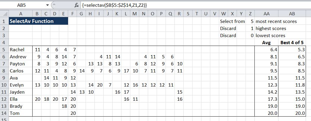
SelectAv function finding the average of the best (lowest) four out of the 5 most recent scores.

The function arguments are:

=SelectAv(DataRange, SelectFrom , DiscardHigh , DiscardLow)

• DataRange: Spreadsheet range containing the data
• SelectFrom (optional): number of values, from the right, to be included.  Blank cells are ignored.
• DiscardHigh (optional): Number of high values to be excluded from the average
• DiscardLow (optional): Number of low values to be excluded from the average

If all optional values are omitted the function will return the same as the built in Average() function, except that it returns a column array, with one value for each row of the selected data range.  The function must be entered as an array function, using Ctrl-shift-enter.  See https://newtonexcelbach.wordpress.com/2011/05/10/using-array-formulas/ for details.

The example spreadsheet (including open source code) can be downloaded from: SelectAv.xlsb