Reviewing some of my less visited links recently, I was intrigued by a post at The Math Less Travelled:

The previous post at the site provides more details of the source of the curve, and some links to an interactive curve generator written in Python, using the Jupyter Notebook. I hadn’t heard of the Jupyter Project, and I will certainly be taking a closer look in the future, but for now I thought I would have a go at creating the curve generator in Excel, which turned out to be surprisingly easy, with no coding required.

The curve is defined by the equation:

which looks fairly mysterious to a non-mathematician, but as explained at this Wikipedia article the function consists of three circles in the complex plane, which can be translated into the XY plane with two functions:
x(t) = cos(t) + cos(6t)/2 + cos(-14t)/3
y(t) = sin(t) + sin(6t)/2 + sin(-14t)/3

I have generated these values in Excel in three stages so each component of the curve can be plotted separately, and we can also add a fourth level, as shown in the screenshot below:

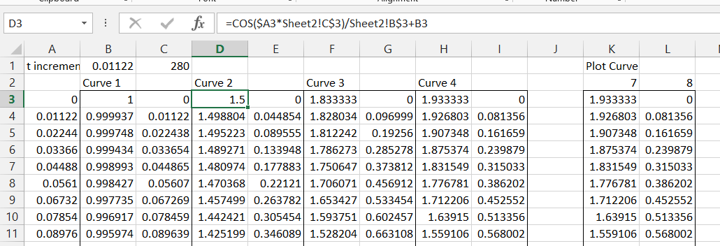
The t values in Colum A simply increment by the value in Cell B1 (set to pi/280 in this example).  The x and y values for Curve 1 are Cos(t) and Sin(t), and the values for Curve 2 (as shown in the formula bar for the x value) are:
=COS($A3*Sheet2!C$3)/Sheet2!B$3+B3
=SIN($A3*Sheet2!C$3)/Sheet2!B$3+C3

The links t0 Sheet2 allow the factors for the curve to be easily changed.  The formulas for Curve 2 can then be copied across for Curve 3, and an additional Curve 4 is added.  The formulas in Row 3 are then copied down as far as required.  Finally the actual values to be plotted are extracted in Colums K and L with:
=INDEX($B3:$I3,K$2)
=INDEX($B3:$I3,L$2)
which are also copied down to cover the full range.

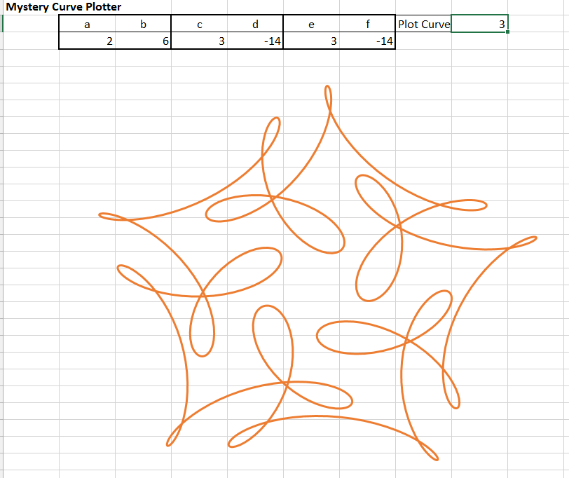
Finally values are entered in the appropriate cells on Sheet 2, and the values in Columns K and L are plotted as an XY (Scatter) chart on Sheet 2, resulting in:

We can now experiment with different curves simply by entering different values under a to f, and choosing which curve to plot. Entering the same factors as c and d under e and f, and selecting curve 4 generates:

Changing the sign for factor f:

And increasing the value of e:

The spreadsheet can be downloaded from MysteryCurve.xlsx.
No open source code this time, because there is no code.
Feel free to add slider bars and animation!

Update:

If you wondered why my plot looks a bit different to the one in the link, it’s because I didn’t get the function right; the third term is multiplied by i/3, not 1/3.  That makes it a bit more complicated, but it can still be done in code-free in Excel.  I have updated the spreadsheet using the functions Complex(), IMProduct(), IMExp(), IMReal(), and Imaginary().  See the download spreadsheet for details, or just enjoy the corrected image below: