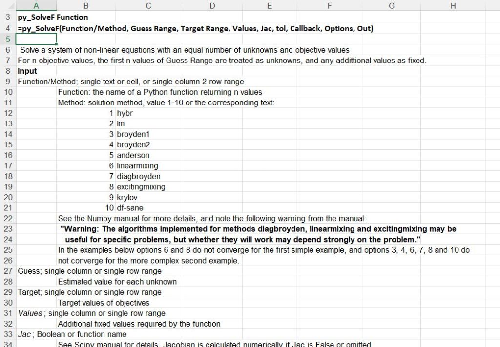
Following the previous post I will continue to look at the py_Solvers spreadsheet included in the download file:

py_SciPy.zip

Details of the required pyxll package (including download, free trial, and full documentation) can be found at: pyxll

For those installing a new copy of pyxll, a 10% discount on the first year’s fees is available using the coupon code “NEWTONEXCELBACH10”.

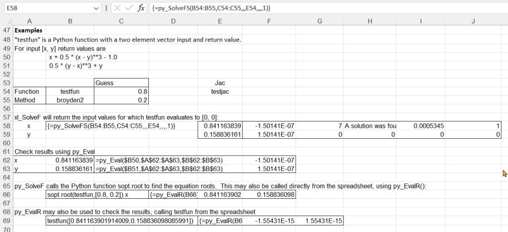
This post will look at the py_SolveFS function for solving multi-variable equations using the Python root function.

Documentation is given on the spreadsheet:

The first example is a simple problem from the Scipy documentation:

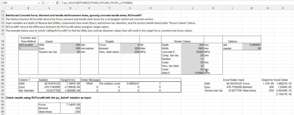
This is followed by a more useful example, looking at the elastic design of a reinforced concrete section. (click on any image for full-screen view):

This is an extension of the second example for the py_Brent function in the previous post. In that case the area of the tension reinforcement was specified, and the depth of the section neutral axis was found for a specified bending moment and axial load. In today’s example only the number of tension bars is specified and the required outputs are the diameter of the tension bars, the strain at the compression face, and the depth of the neutral axis, for a specified bending moment, axial load and tensile stress in the tension reinforcement.

Note that the same results can be generated using the Excel solver:

To solve this problem with the Excel solver the square of the deviation of each return value from the target values is calculated on the spreadsheet, then the sum of the squares is minimised, The Excel solver solution is identical to the Python results, but it has several disadvantages:

• It is slower
• It takes longer to set up
• It is less flexible and provides less control over solution methods
• The solver results need to be recalculated every time an input is changed

The final example is a more complex problem from the Scipy docs (see the docs for full details):