Many of the user defined functions (UDF’s) presented in this blog return an array rather than a single value. Options for displaying arrays in Excel have changed significantly in recent years and this post looks at the most efficient ways of working with these changes, including some situations when the old way is still the best.

In addition to the built-in Excel options, using Python code via pyxll allows large multi-dimensional arrays to be passed to Excel as a cache object, which has significant advantages in some situations. This will be covered in more detail in the next post.

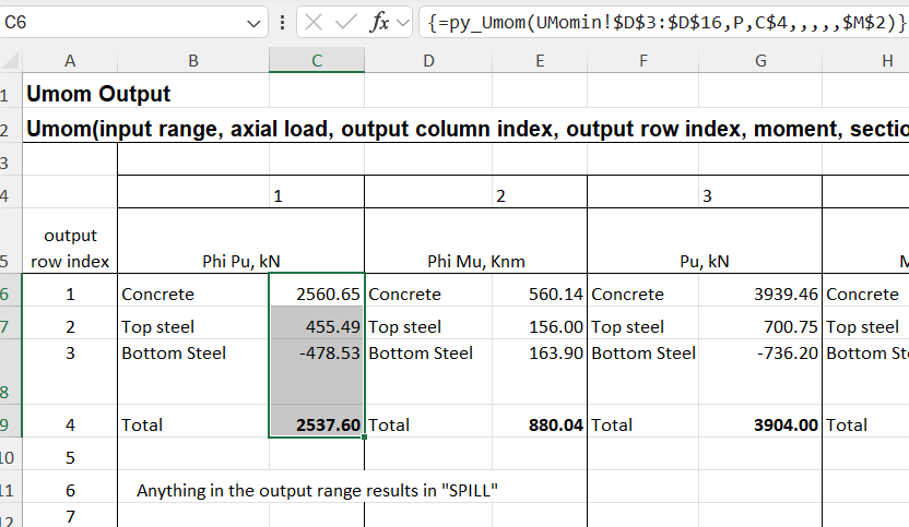
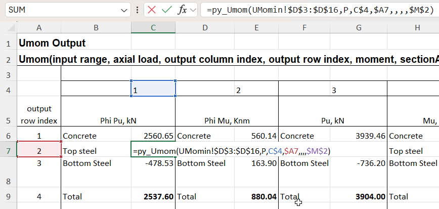
The screenshot below shows output from the py_Umom UDF entered as a fixed array:

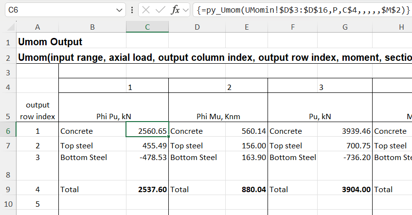
The function shown in cell C6 returns a column array. In old versions of Excel only the first cell is returned, but in recent years “dynamic arrays” have been introduced, which automatically display the whole array. Either way, the array can be entered to display fully or in part with the following steps:

• Enter the function in the top cell and press enter in the usual way
• Select the range of cells to be displayed, in this case C6:C9
• Press F2 for edit mode, then Ctrl-Shift-Enter

The function will then display as above, with values in the selected cells, and the function encased in braces, {}, in the edit line.

It may be desired to return to the default display, either to change the extent of the displayed array in any Excel version, or to display the full dynamic array in recent versions. In that case:

• Select the top cell and press F2 (edit mode)
• Press Ctrl-A to select all the formula text:

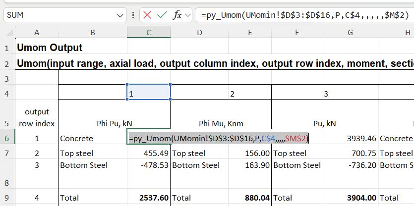
• Press Ctrl-X to cut the formula and copy to the clipboard
• Press Ctrl-Shift-Enter

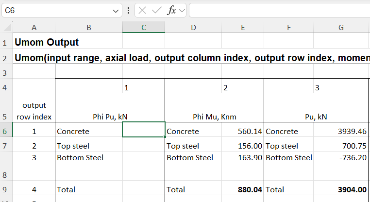
• All the cells will now be empty
• With the cursor still in cell C6, press Ctrl-V to re-paste the formula

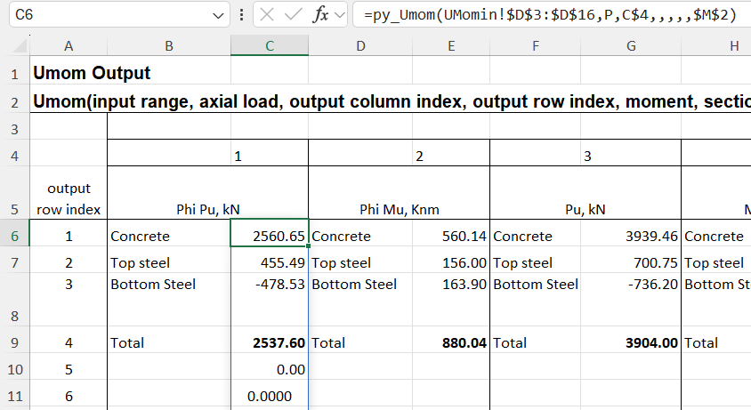
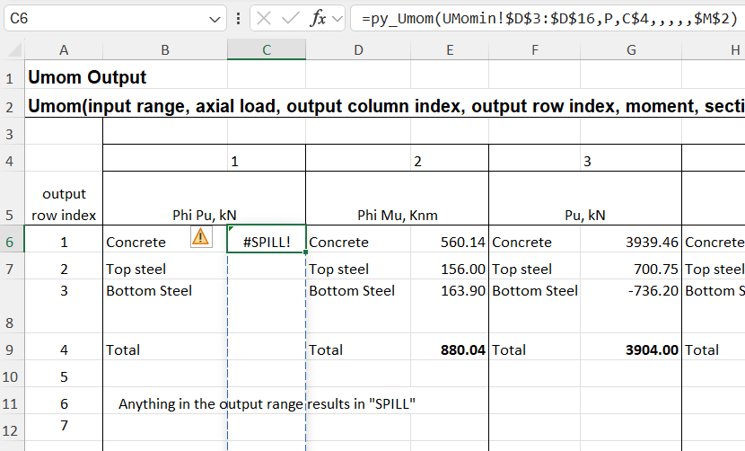
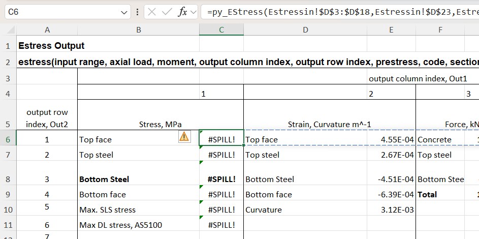
In this case the dynamic array returns zeros in multiple cells below the desired results. One problem with this, other than appearance, is that if any text is entered in a cell in the output range, the entire output will change to “#SPILL!” in the top cell, with all the others displaying as blank:

The only way to fix this whilst maintaining the dynamic array is to change the UDF code to remove the empty cells before they are returned to Excel. Alternatively, do it the old way and:

• Select the desired output range
• Press F2
• Press Ctrl-Shift-Enter

An alternative for the py_Umom function is to enter the Offs2 input, which specifies the row number, with that row being returned a single value:

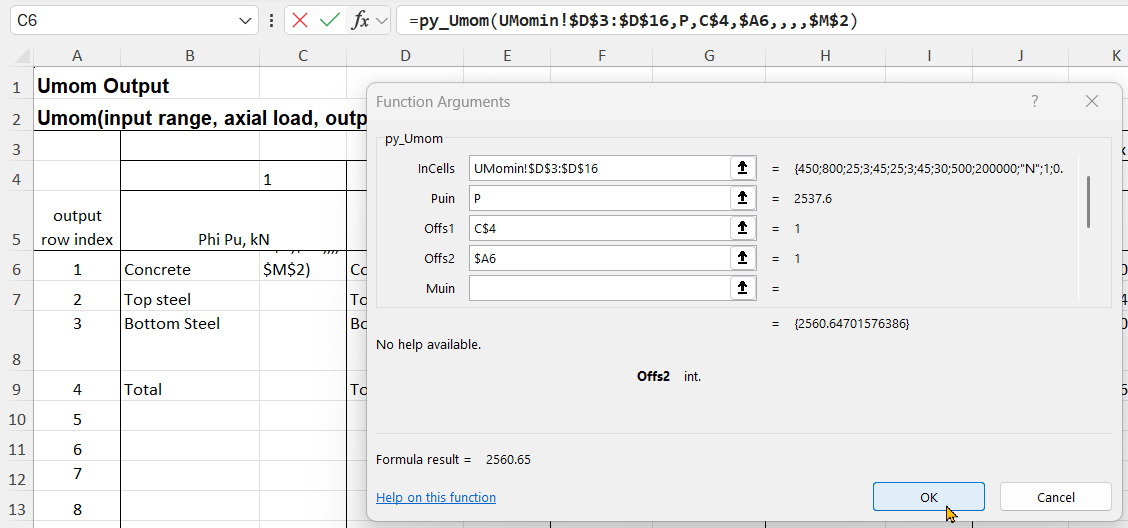
The formula is entered with the Enter key, which displays the single value, without the {}.

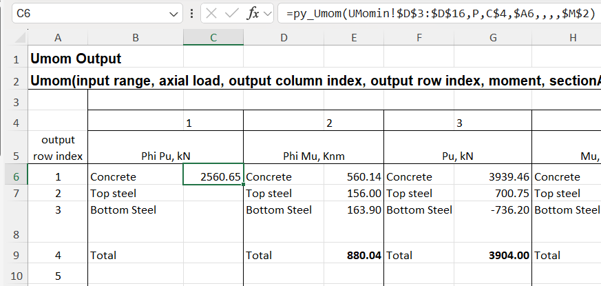
With Offs2 entered as a relative address, with no $ before the 6, the formula can then be copied to the other 3 rows:

The py_Estress function currently works differently, when the output row is defined it returns a row array with the chosen result in the first cell, and other unwanted data in the rest. This is not a useful feature, but it’s a work in progress. When the function is entered as a dynamic array recent versions of Excel will return the whole row, but just display #SPILL! if any of the cells in the output range are not empty:

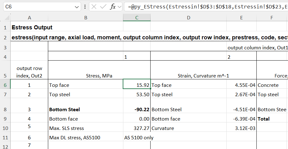
The first cell can be displayed with Ctrl-Shift-Enter, but an alternative that may be preferred, and is often inserted automatically by Excel, is to insert @ at the start of the formula, known as the “implicit intersection operator”. This has different behaviour when used on Excel tables of ranges, but for a range returned by a UDF, either VBA, Python, or any other code, it returns the first value of the array, or the top-left for a 2D array:

More details of the @ operator can be found at the Microsoft Site.

As far as I know, Ctrl-Shift-Enter is the only built-in way to display part of an array returned by a UDF, and the displayed results have to start at the top-left. Alternative options using the pyxll cache object will be discussed in the next post.