In the final post in this series I will look at linking Excel to the Scipy special, distance, space and constants functions and also the Fast-Fourier Transform (FFT) functions.
The py_Special-Dist and py_FFT spreadsheet, with associated Python code in PythonSpaceFuncs3.py and pyScipy3.py, are included in the download file. There have been significant changes since the previous post, so download the latest version at:
Details of the required pyxll package (including download, free trial, and full documentation) can be found at: pyxll
For those installing a new copy of pyxll, a 10% discount on the first year’s fees is available using the coupon code “NEWTONEXCELBACH10”.
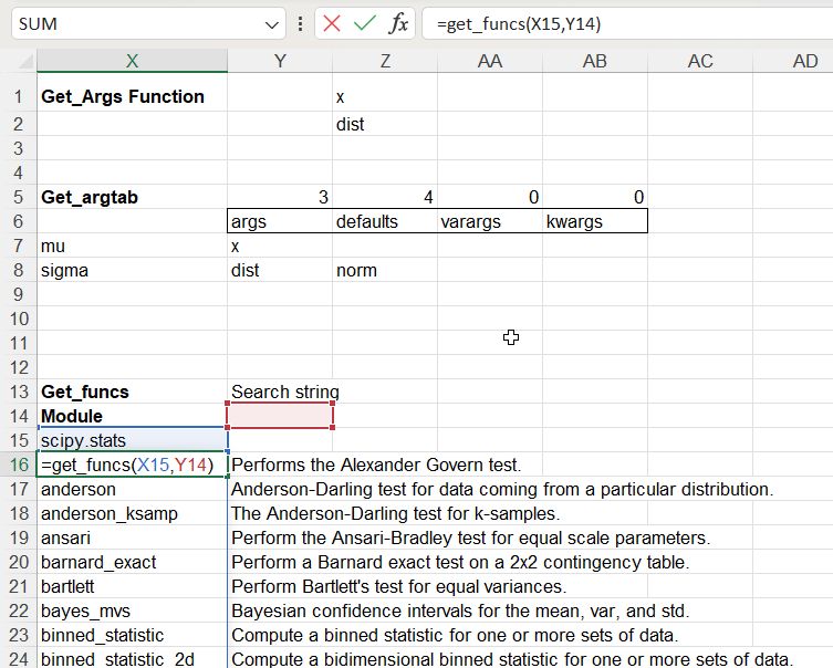
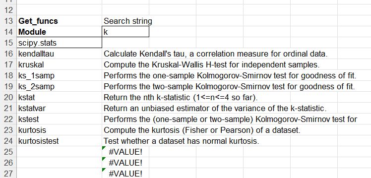
The coded Scipy documentation can be displayed in Excel, using the get_docs function:

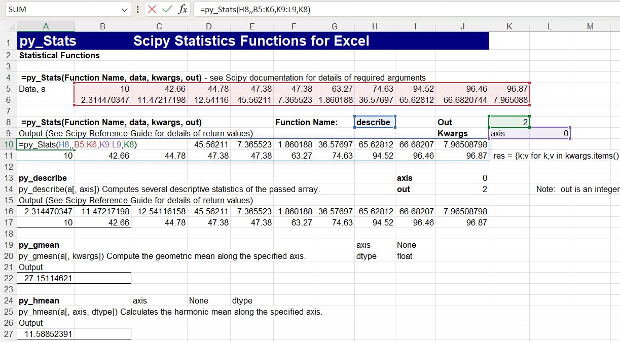
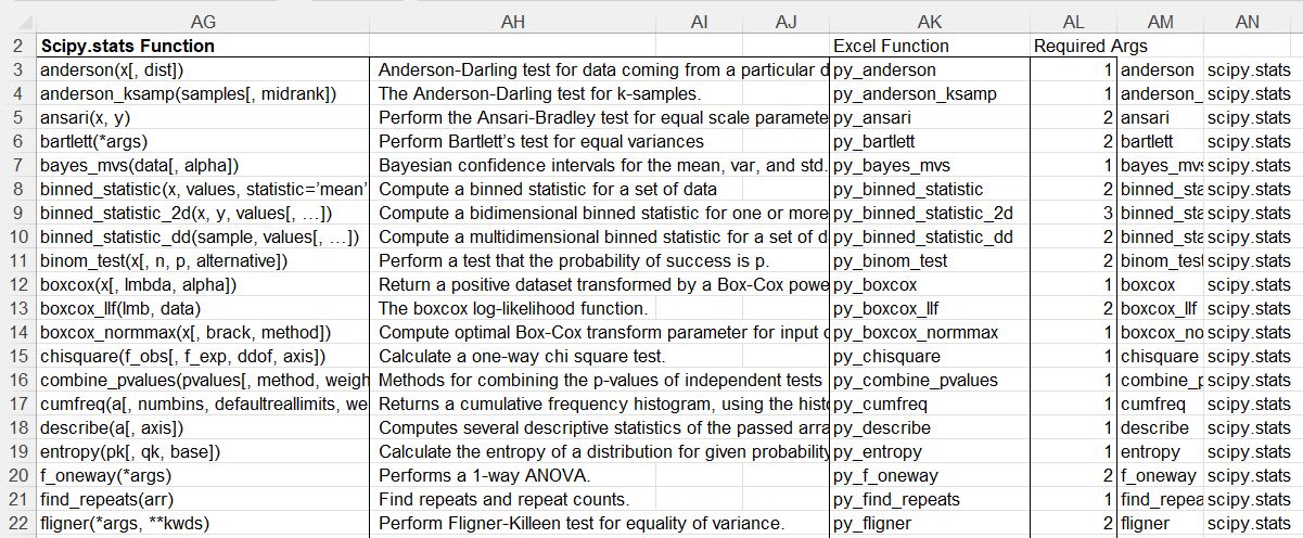
The Scipy special functions are called with the py_CallfuncS function. The spreadsheet lists the 220 available functions with a description, and is set up to generate simple examples:

The Distance worksheet shows alternative methods to call the distance functions:

The Space worksheet has examples of the py_Delaunay, py_ConvexHull and py_Voronoi functions:

The Scipy constants return a range of physical constants, including definition of units, accessed with py_GetConst:

The NIST CODATA constants can be accessed with the py_GetCodata function:

The py_FFT spreadsheet has an example from the Scipy documentation, using the functions py_fft, py_fftfreq, and py_ifft:

The FFT results are also plotted using Matplotlib with the py_plot function:

More information on using Matplotlib with Excel can be found at: