My Windows search function recently once again stopped indexing pdf files, probably associated with an upgrade to Windows 11. Previously this was fixed by downloading the file PDFFilter64Setup.msi from the Adobe site, but that download no longer works, and there is nothing useful from Adobe or from Windows help. After much searching I eventually found a Wikipedia article with a working link:
In A not so easy problem I looked at using Python with Excel (via pyxll) to work with very long integers, using the MPMath package. For high precision calculations involving decimal values MPMath is required, but for simple operations entirely on integers the native Python integers can be of any length, so this post looks at using Python integers from Excel. The examples below have been added to the py_Numpy spreadsheet, which can be downloaded with the associated Python code from:
Note that the Python code comes in two version, with or without calls to the Numba just-in-time compiler. I am currently using the latter, since the standard installation of Numba does not yet support Python 3.11.
The first example uses Python integers to return the factors of integers of any length:
The function returns the factors of any given integer, followed by the calculation time. The first example (row 6) took about 20 seconds to return the results, so has been converted to text, but the example on row 9 is any active function, which takes less than 0.08 seconds to run.
The factorization function calls gcd(), which returns the greatest common divisor of two integers, and can be called from Excel using py_gcd:
The two integers are passed as strings (since Excel can’t handle very long integers), then converted to integers and passed to gcd(). The integer return value is than converted to a string for return to Excel.
Three functions are provided for integer division:
int_mod(n1, n2) returns the remainder of n1 divided by n2. The example confirms that 112969501600351915928116 is indeed an exact factor of 11193123069125255733930404403495413078162092382549228
int_floor(n1, n2) returns the integer part of n1, divided by n2, using the Python // operator, whereas int_div(n1, n2) returns the complete result of the division, including any decimal part, using the / operator. Note that division of two integers using / in Python always returns a float, even if the divisor is an exact factor, as in this case. The code returns the resulting value to Excel as a string, but all digits after the 16th are lost. To retain the full precision with long integers use the int_floor function.
The multiplication, addition and subtraction functions are more straightforward, since the results of these operations will always be another integer:
I have now converted my ULS Design Functions spreadsheet (last presented here) to Python. The new spreadsheet and open source Python code can be downloaded from:
The spreadsheet has the same functionality as the VBA version, providing ULS analysis of any reinforced concrete section divided into trapezoidal layers, to Australian codes, Eurocode 2, and ACI 318. It also has the added functionality of design for shear (currently to Australian codes only), and a function allowing simplified input for rectangular sections.
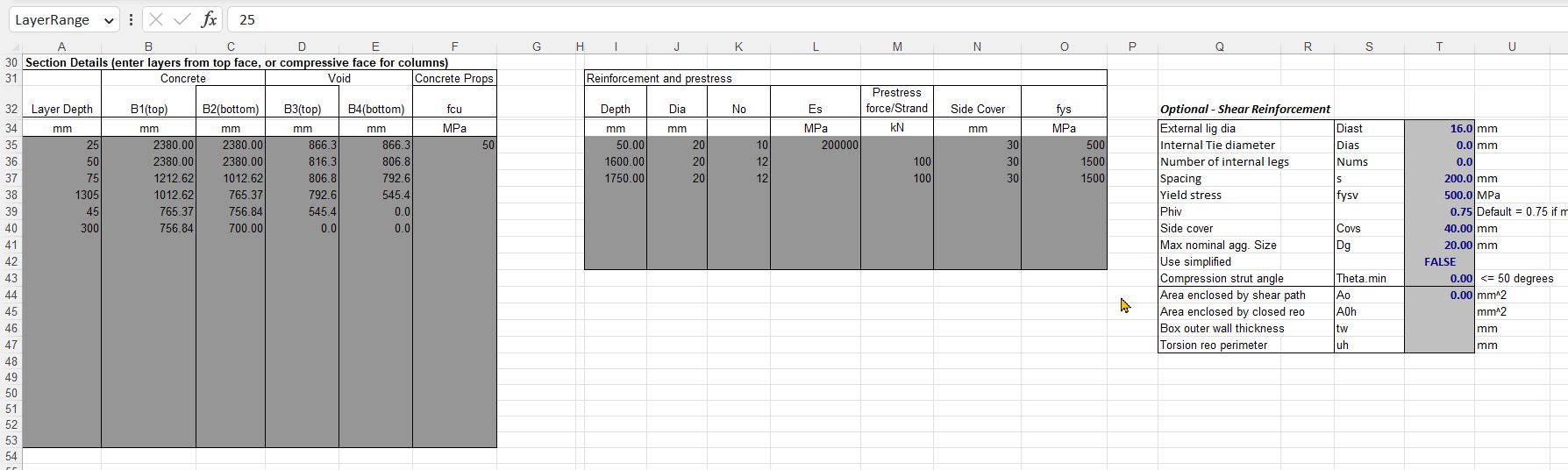
Input is in the same format as the VBA version, with the optional addition of shear data input where required (click any image for full-size view):
Note that for shear design:
The design shear force and torsion, and the associated bending moment must be entered in the range D5:F5.
For any hollow or non-rectangular section, or a section with prestressing ducts, the effective web width must be entered in cell F8.
For box sections the additional data in range T44:T47 is required.
The tendon angle entered in cell F9 is currently only used for shear design.
Output is also in similar format, with the addition of shear related results:
The py_UmomR function has simplified input for rectangular sections with two layers of reinforcement:
A list of files available for free download can be found under the Downloads link at the top of the page:
The list has now been updated and there are now 189 files available for download, most with open source VBA and/or Python code.
The list is in Excel worksheet format, and can be displayed in full-screen view by clicking on the icon in the bottom-right corner:
The list can be sorted by any of the columns, and has hyperlinks to download the file (Column A) and to the latest blog post featuring the file (Column B):
Note that the linked blog posts also have download links, but those from early 2019 or before will often be in http: format (rather than https:), which will not work with modern browsers. In that case just return to the download list, where all the links should work.
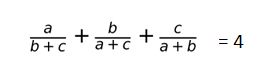
Checking the results is not so simple either. The values have up to 80 digits, which is way beyond the standard precision available in Excel, but using the Python mpmath library, with the EvalU spreadsheet, it can be done. Enter the three values as text (or copy and paste!), enter the formula, set the number of significant figures to 85 or more, and use the mp_Eval function:
Changing the last digit of one of the values confirms that the evaluation is working to the required precision: