Time to Lookup

At Daily Dose of Excel Jeff Weir has been looking at alternative methods of applying the VLookup function and ways of getting precise timing of the different formulations.

Based on his posts there I have written two Lookup User Defined Functions (UDFs):

  1. The LookExact Function finds the nearest lower match to a lookup value from a list of sorted data, then checks if this value is exactly equal to the lookup value (or optionally within any specified tolerance).  The advantage of this approach over using the built-in VLookup function with the “Approximate Match” option set to false is that a binary search on sorted data (as performed when the “Approximate Match” option is set to True) is hugely faster than searching through the list from beginning to end.
  2. The LookNear function also   performs a binary search to find the nearest lower match to the lookup value, then checks the next value from the list, and returns the closer value.

Checking the performance of these functions revealed some surprising differences, which in some cases turned out to be more to do with the method of timing than real differences between the various formulas and VBA routines, so I have also added my own version of the timer routines published at: speed performance measure vba function.

A spreadsheet including the Lookup functions and timer routines can be downloaded from: ExactLookup.zip, including full open source code and some example timings as discussed below.

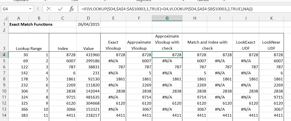
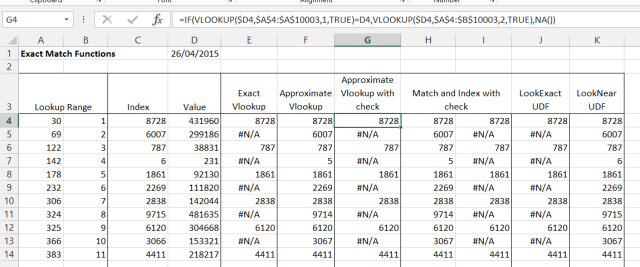
Four alternative lookup formulas, and the two UDFs are tested in the spreadsheet, as shown in the screen shot below:
ExactLook1

The lookup range in the download spreadsheet consists of 10,000 sequential numbers in column A, with an index value in column B.  The formulas have also been checked on a table of 1 million rows.  Column C contains 200 index values used to generate the values in Column D, using the formulas:

  1. =Index(A$4:A$10003, C4)
  2. =Index(A$4:A$10003, C5) + 1
  3. =Index(A$4:A$10003, C6)
  4. =Index(A$4:A$10003, C7) – 1

These four formulas were then copied down 200 rows to generate values that were alternately an exact value found in the lookup table, or just over or under one of the exact values.  Having generated the list the formulas were then converted to values.

Columns E to K contain:

  1. E: Exact Vlookup –  =VLOOKUP($D4,$A$4:$B$10003,2,FALSE)
  2. F: Approximate Vlookup – =VLOOKUP($D4,$A$4:$B$10003,2,TRUE)
  3. G: Approximate Vlookup with check –
    =IF(VLOOKUP($D4,$A$4:$A$10003,1,TRUE)=D4,VLOOKUP($D4,$A$4:$B$10003,2,TRUE),NA())
  4. H,I: Match and Index with check –
    =MATCH(D4,$A$4:$A$10003,1)
    =IF(INDEX($A$4:$B$10003,H4,1)=D4,INDEX($A$4:$B$10003,H4,2),NA())
  5. J: LookExact UDF – =LookExact($D$4:$D$203,$A$4:$B$10003,2)
  6. K: LookNear UDF – =LookNear($D$4:$D$203,$A$4:$A$10003,$B$4)

For the rows where the lookup value is an exact match to a value in the lookup range all the formulas return the same result (the index number from column B).  Where there is no exact match formulas 1, 3, 4, and 5 return #N/A, as intended.  Formula 2 returns the index number for the last row that is less than the lookup value, and Formula 6 (LookNear) returns the index number for the row that contains the value closest to the lookup value.

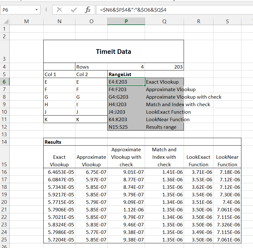
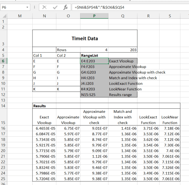
The screenshot below shows the input for the Timeit routine, and typical results:
ExactLook2

The required input is the two grey shaded columns.  The first column lists the ranges containing formulas to be timed.  Normally each range will have the same number of rows, but this isn’t necessary.  The table has been set up to generate the range addresses from the adjacent row and column details, but the ranges can also be just typed in as text.  The second column contains a description of each of the formulas.  The final row of column 1 contains the address for the output results, which should be 11 rows x one column for each formula range.

The range list may be extended (or reduced) as far as required.  If the number of rows is changed, or if the list is moved, the range name “RangeList” must be adjusted to suit.

Note that the extent of the array functions in columns J and K must be adjusted to match the recalculation ranges listed in P10 and P11.   To do this:

  • Edit the first cell in each column so that the first argument (“lookval”) covers the required number of rows.
  • Re-enter by pressing Ctrl-Shift-Enter.
  • Re-size the array extent by pressing Ctrl-Shift-S, which calls the custom  SetArrayToNaturalSize routine.

The Timeit routine recalculates each of the listed ranges 10 times, and generates a table of recalculation times in seconds per row.  To run the routine press Alt-F8 and select Timeit.

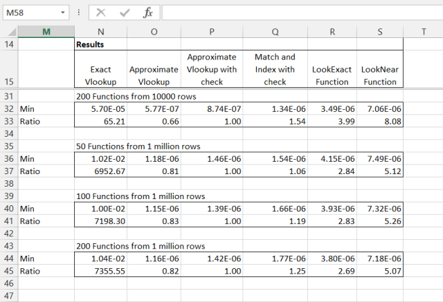
Typical results for a range of lookup table sizes and number of functions are shown below:
ExactLook3

It can be seen that the “Exact Vlookup” formula is by far the slowest, and with the long table it is over 7,000 times slower than the “Approximate Vlookup”.

The “Approximate Vlookup” is the fastest, but if the formula is required to return #N/A if there is no exact match, then the “Approximate Vlookup With Check” formula was surprisingly fast, taking only 25% longer on the long tables.

Splitting the formula into two columns, and using the Match and Index functions was, surprisingly, slower than the equivalent using Vlookup.

The two UDFs were slower than the Approximate VLookup formulas, but since the calculation time was only 4 to 8 microseconds, even with the 1 million row table, this would only become significant for enormous tables.

Posted in Arrays, Excel, UDFs, VBA | Tagged , , , , , , | 5 Comments

John Renbourn; 1944 – 2015

John Renbourn

John Renbourn, who has died aged 70, was one half of the powerful guitar duo of Pentangle, the innovative jazz-folk band of the 1960s and 70s. While his fellow guitarist, Bert Jansch, brought great emotion and inventiveness to his playing, it was Renbourn who provided a high level of technical accomplishment. They revelled in one another’s virtuosity.

Posted in Bach | Tagged , | Leave a comment

Re-sizing Array Functions

The recent updates to the ConBeamU spreadsheet contained two new functions for entering and re-sizing array functions, and since they will be useful on any spreadsheet containing array functions (which here means almost all of them) I thought they deserved a blog post of their own.

I have added the new functions to the CSplineA spreadsheet, which can be downloaded from:

CSpline2.zip

The code for the new functions was taken from: Technicana .  The only changes I have made are:

  1. If the original function failed for any reason the array function being re-sized was deleted.  I have added a couple of lines so it will be re-written back to the spreadsheet.
  2. I have changed the shot-cut codes as detailed below.

To use the functions start by entering any function that returns an array in the top-left corner of the desired output range:

resize-1

To expand the function to display the full extent of the array, press Ctrl-Shift-S:

resize-1a

To re-size the array select the required range and press Ctrl-Shift-R:

resize-2

To move the array to a range overlapping with the original range (with the new range to the right and/or below the original), select the top left cell of the new range then press Ctrl-Shift-S (for the full array), or select the output range required and press Ctrl-Shift-R:

resize-3

If the destination range is either to the left of, or entirely outside, the original range then the array function must first be copied to the top-left cell of the destination range, then proceed as above.

A word of warning: the functions clear the undo stack, and will write over any data in the output range without warning, so if there is any danger of the output range writing over any data you need, save your work before proceeding.

Posted in Arrays, Excel, UDFs, VBA | Tagged , , , , , , | 4 Comments

ConbeamU Update Update

Following some comments from 4Step on the last ConbeamU update, and a thorough check of results against Strand7 results, I have posted a new version that fixes a number of issues with the previous one.  The new version number is 4.01, and it may be downloaded from:

ConBeamU.zip

The file is a free download, and includes full open-source code.

The download zip file also contains a summary of the check runs performed with the Strand7 finite element software. In Strand7 I have set up a model with 15 separate continuous beams, with the same loading but different support conditions, ranging from a single cantilever to a 3 span beam with cantilevers at both ends. These beams have been analysed in Strand7 and ConbeamU with different restraints applied at each support, and the results are compared in the Check Conbeam spreadsheet included in the zip file. The results show near exact agreement in all cases.

Continuous beams model in Strand7

ConbeamU4-1

Strand7 Results

ConbeamU4-2

Strand7 and ConbeamU results compared in Check Conbeam.xlsb

ConbeamU4-3

Posted in Beam Bending, Excel, Frame Analysis, Newton, Strand7, UDFs, VBA | Tagged , , , , , | 4 Comments

ConbeamU Update; defined support deflections

As promised in a recent post, I have updated the ConBeamU spreadsheet to allow defined deflections to be specified at any support.

The new spreadsheet (including full open-source code), can be downloaded from ConBeamU.zip

In addition to the support deflections the new spreadsheet has the following changes:

  • In addition to providing a list of output point positions it is now possible to specify the number of points required for each span.
  • At support positions output is now provided for the shear and moment on either side of the support.
  • VBA routines are now provided to simplify the entry or re-sizing of array functions.
  • Behind the scenes, the VBA code has been re-arranged to allow many of the functions to be used in the frame analysis spreadsheets, reducing duplication of code.

Defined support displacements and the new input of output points is shown below:

ConbeamU3-1
The output from this data is similar to the previous version, except that output X values are included in the output:

ConbeamU3-2

The output points may also be defined from a list as in the previous version:
ConbeamU3-3

ConbeamU3-4

Note that where the same output point is defined twice, at a support or point load position, the output now returns the shear force and moments immediately to the left of the point, followed by the values immediately to the right.

The array entry routines are illustrated below.  Any of the functions may be entered in a single cell:

ConbeamU3-5

Then press Ctrl-Shift-S, and the full array will be returned automatically:

ConbeamU3-6

The array range may also automatically be reduced in size.  Select the required output range and press Ctrl-Shift-R:

ConbeamU3-7

More details of the array entry routines are provided on the spreadsheet:
ConbeamU3-8


Posted in Arrays, Beam Bending, Excel, Frame Analysis, Newton, UDFs, VBA | Tagged , , , , , , , , , | 12 Comments