I recently upgraded to Python 3.12, and installed the latest version of the Numba just-in-time compiler (0.60.0) which also required upgrading Matplotlib (3.9.3), and downgrading Numpy (2.0.2). I have also edited calls to Numba in the py_3DFrame1_1.py module, and added this to the download file at:
See Installing 3DFrame-py for installation details, and details of other Python modules required. Also see Python and pyxll for details of the required pyxll package, including a coupon code for a 10% discount.
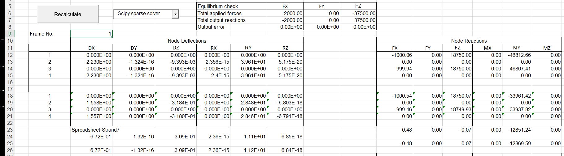
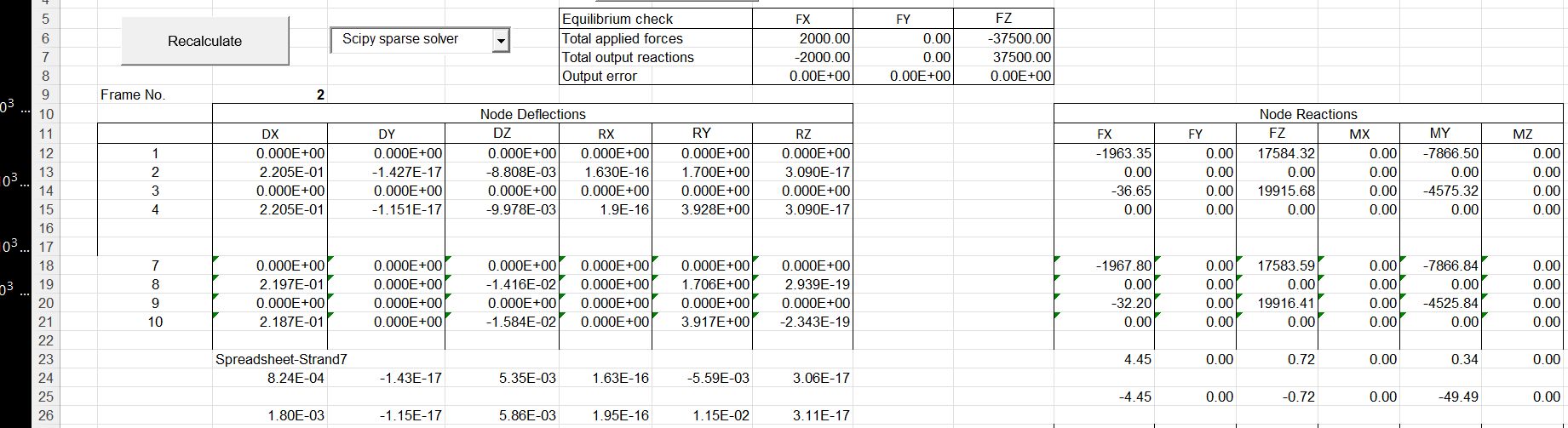
The name of the currently active 3DFrame module is now shown on the Output sheet:

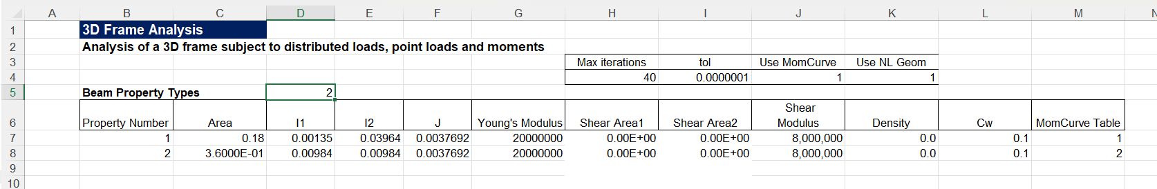
To change to the Numba version, enter 1 in cell E3, then click Reload Solvers, and update the function in cell H3:

If the “reload solvers” button doesn’t work, save the file, close Excel and restart, and the selected module will load.
The Numba compilation process takes about 15 seconds, and is required every time the file is opened, but for very large models the Numba code is significantly faster; for instance calculation time of the 3DFrame-py-vvbig.xlsb model, with over 27,500 beams, is reduced from 17.7 seconds to 6.6 seconds.
One other minor code change fixed a problem with data copied from the VBA version of the 3DFrame program. The input for the beams had left the rotation angle column blank. This is treated as zero in VBA, but when imported through a Numpy array into Python it is converted to NAN. This can be dealt with by a single line of code:
BeamCon[np.isnan(BeamCon)] = 0