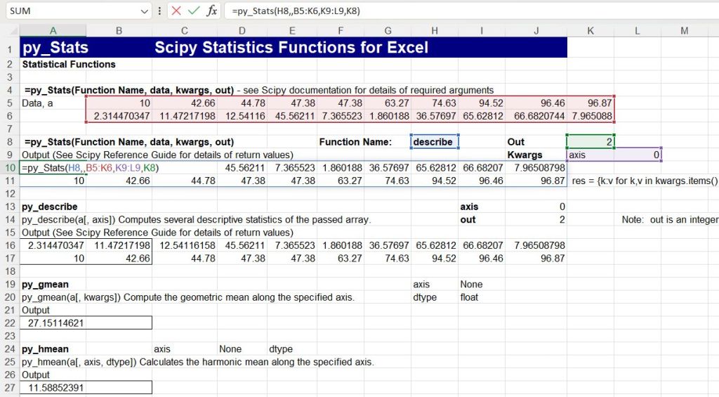
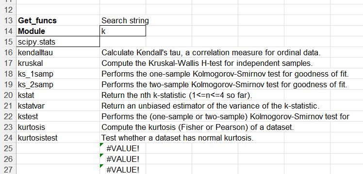
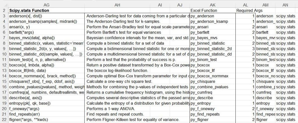
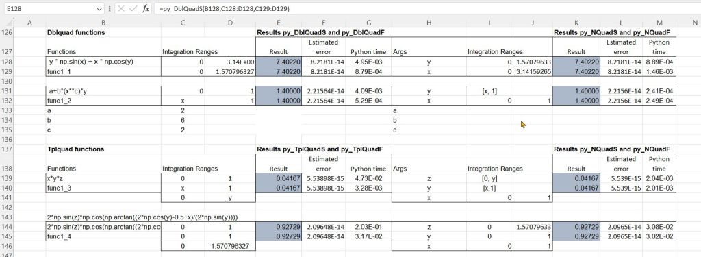
Scipy Functions with Excel and pyxll 3 – Solvers 1

Following the the first post in this series I will move on to the py_Solvers spreadsheet included in the download file:

py_SciPy.zip

Details of the required pyxll package (including download, free trial, and full documentation) can be found at: pyxll

For those installing a new copy of pyxll, a 10% discount on the first year’s fees is available using the coupon code “NEWTONEXCELBACH10”.

This post will look at functions for solving equations with one variable, and the next one multi-variable equations.

The py_Brent function finds a root to a function of one variable within a specified range using Brent’s Method:

The function may either be entered as text on the spreadsheet using the Python lambda format, or may be the name of any accessible Python function. In the example above func2 and func3 are included in the pyScipy3 module:

def func2(x):
    return -2*x**4 + 2*x**3 + -16*x**2 + -60*x + 100

def func3(x, a, b):
    return -2*x**4 + 2*x**3 + -16*x**2 + -a*x + b

The py_BrentA function allows two of the function arguments to be transferred as row and column arrays, with the result returned as a table:
In the first example the function has one unknown, T, two variable arguments, epsilon and alpha, and five fixed arguments, G_1 to G_5. 

The 5 fixed arguments have been converted to numerical values using the py_Eval function so that the unknown and the two variable arguments are the only arguments required for the py_BrentA function:

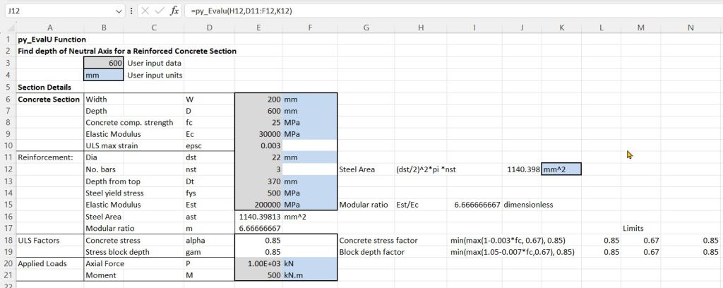
The second example finds the depth of the Neutral Axis of a reinforced concrete section with elastic properties with two variable arguments (applied axial force and bending moment) and 7 fixed arguments

For the on-sheet lambda function the fixed arguments must be converted to numerical values, again using py_Eval, but for the Python function the values can be passed to the function as an array:

def FindDNA(x, Ax, Mom, addargs):   
 
    A = addargs[0]
    B = addargs[1]
    C = addargs[2]
    D = addargs[3]
    E = addargs[4]
    F = addargs[5]
    G = addargs[6]
    
    ecc = Mom*1000/Ax
    
    return A*x**3+(B-C*ecc)*x**2+(D-ecc*E)*x+Mom*1000/Ax*F-G

On the spreadsheet either approach may be used by entering 1 or 2 in the “Func Type” cell (Y74).

The py_MinimizeFS function has similar functionality to py_Brent, but uses the Python minimize_scalar function, that allows alternative solver methods:

The py_MinimizeF function provides unconstrained or constrained minimization of scalar functions of one or more variables using the Python minimize function, using 11 alternative solver methods. 

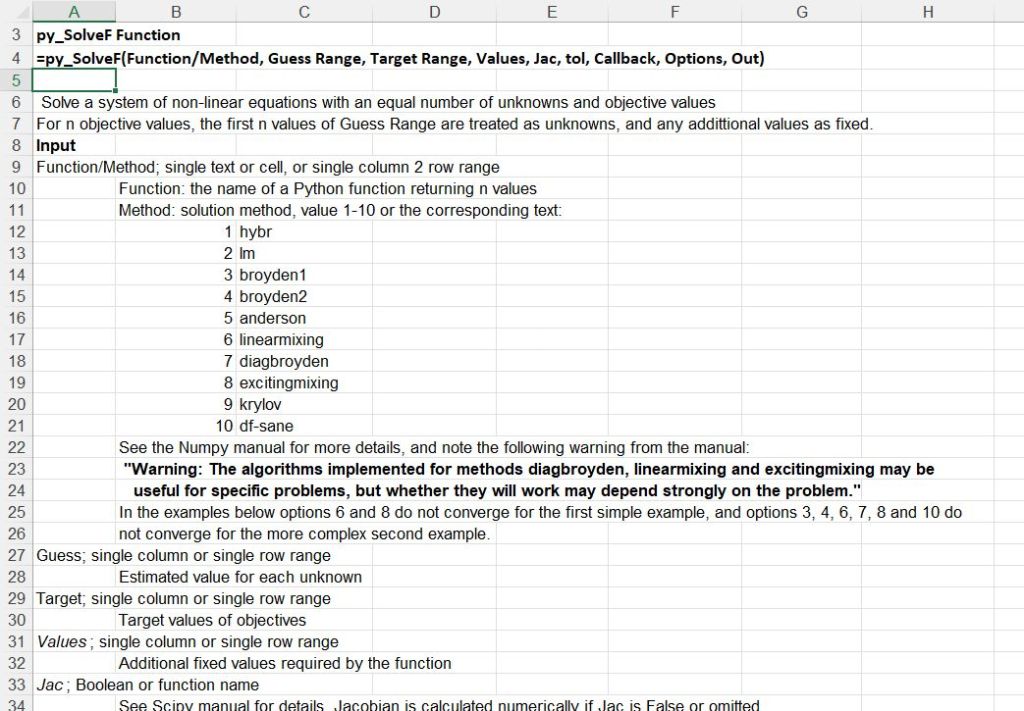
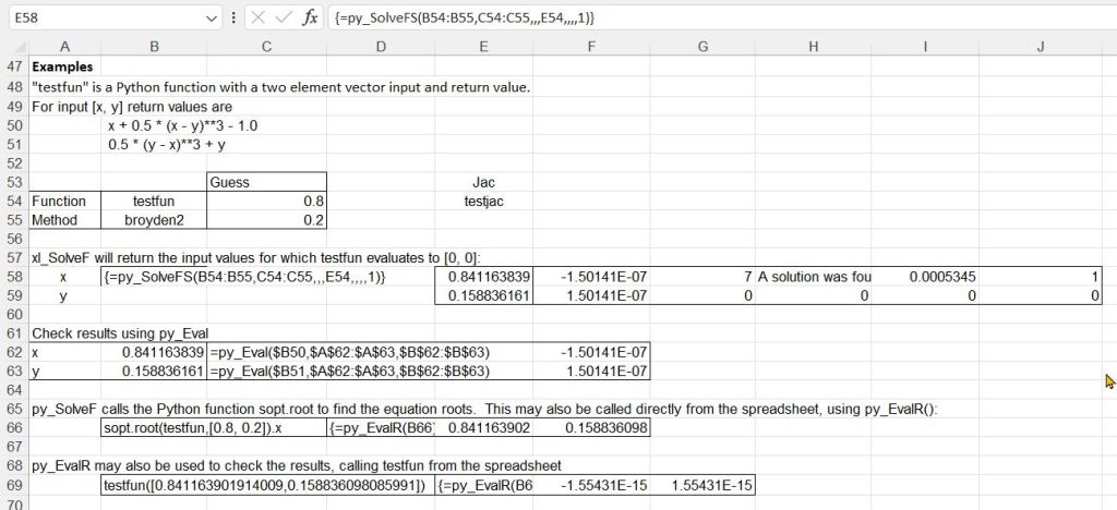
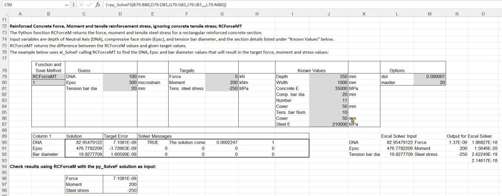
The py_FindRoots function returns a root of a vector function.

Examples in the spreadsheet include the root finding example used for the py_Brent function, and more complex examples from the Scipy documentation:

Posted in Excel, Link to Python, Maths, Newton, NumPy and SciPy, PyXLL, UDFs | Tagged , , , , , , , , | Leave a comment

Scipy Functions with Excel and pyxll 2 – Interpolation

Following the previous post I will now look in more detail at the functions in the py_Interpolate spreadsheet included in the download file:

py_SciPy.zip

Details of the required pyxll package (including download, free trial, and full documentation) can be found at: pyxll

For those installing a new copy of pyxll, a 10% discount on the first year’s fees is available using the coupon code “NEWTONEXCELBACH10”.

The py_Interpolate spreadsheet has 10 user defined functions linking to the Scipy spline interpolation functions. The Scipy help on each function is easily accessed from within Excel:

Open the “Insert Function” dialog, then click on “Help on this function” in the bottom left corner.

That takes you straight to the Scipy on-line help:

The examples in the spreadsheet plot the same data using each of the 9 functions. The screenshots below compare the output from the py_CubicSpline function, with “natural” end conditions, with the other nine functions:

py_Akima1D:

py_BarycentricInterp:

scipy.interpolate.barycentric_interpolate

scipy.interpolate.barycentric_interpolate(xiyixaxis=0)

Convenience function for polynomial interpolation.

Constructs a polynomial that passes through a given set of points, then evaluates the polynomial. For reasons of numerical stability, this function does not compute the coefficients of the polynomial.

This function uses a “barycentric interpolation” method that treats the problem as a special case of rational function interpolation. This algorithm is quite stable, numerically, but even in a world of exact computation, unless the x coordinates are chosen very carefully – Chebyshev zeros (e.g., cos(i*pi/n)) are a good choice – polynomial interpolation itself is a very ill-conditioned process due to the Runge phenomenon.

py_KroghInterp:

scipy.interpolate.krogh_interpolate

scipy.interpolate.krogh_interpolate(xiyixder=0axis=0)

Convenience function for polynomial interpolation.

See KroghInterpolator for more details.

py_GridData1

scipy.interpolate.griddata

scipy.interpolate.griddata(pointsvaluesximethod=’linear’fill_value=nanrescale=False)

Interpolate unstructured D-D data.

py_UniSpline

scipy.interpolate.UnivariateSpline

class scipy.interpolate.UnivariateSpline(xyw=Nonebbox=[None, None]k=3s=Noneext=0check_finite=False)

1-D smoothing spline fit to a given set of data points.

Fits a spline y = spl(x) of degree k to the provided xy data. s specifies the number of knots by specifying a smoothing condition.

py_Splev

scipy.interpolate.splev

scipy.interpolate.splev(xtckder=0ext=0)

Evaluate a B-spline or its derivatives.

Given the knots and coefficients of a B-spline representation, evaluate the value of the smoothing polynomial and its derivatives. This is a wrapper around the FORTRAN routines splev and splder of FITPACK.

py_CubicSplineS

scipy.interpolate.CubicSpline

class scipy.interpolate.CubicSpline(xyaxis=0bc_type=’not-a-knot’extrapolate=None)

Cubic spline data interpolator.

Interpolate data with a piecewise cubic polynomial which is twice continuously differentiable [1]. The result is represented as a PPoly instance with breakpoints matching the given data.

py_Interp1d(

scipy.interpolate.interp1d

class scipy.interpolate.interp1d(xykind=’linear’axis=-1copy=Truebounds_error=Nonefill_value=nanassume_sorted=False)

Interpolate a 1-D function.

Legacy

This class is considered legacy and will no longer receive updates. This could also mean it will be removed in future SciPy versions.

py_Pchip

scipy.interpolate.PchipInterpolator

class scipy.interpolate.PchipInterpolator(xyaxis=0extrapolate=None)

PCHIP 1-D monotonic cubic interpolation.

x and y are arrays of values used to approximate some function f, with y = f(x). The interpolant uses monotonic cubic splines to find the value of new points. (PCHIP stands for Piecewise Cubic Hermite Interpolating Polynomial).

Posted in Curve fitting, Excel, Link to Python, Maths, Newton, NumPy and SciPy, PyXLL, UDFs | Tagged , , , , , , , , | Leave a comment

Scipy functions with Excel and pyxll

Over the years, I have posted a large number of user defined functions (UDF’s) allowing Python Scipy functions (and related libraries) to be accessed from Excel. These have now been consolidated in a uniform format, using the pyxll add-in and can be downloaded from:

py_SciPy.zip

The download contains full open-source Python code and example spreadsheets that will be reviewed in this and following posts. To use the code the following software is required:

  • Excel for Windows
  • Python
  • Numpy, Scipy, and additional packages for specific applications (see later posts for details)
  • A licenced copy of pyxll (or an active demonstration version)

Details of the pyxll package (including download, free trial, and full documentation) can be found at:

pyxll

For those installing a new copy of pyxll, a 10% discount on the first year’s fees is available using the coupon code “NEWTONEXCELBACH10”.

Having installed Python, Numpy, Scipy and pyxll:

  • Copy the contents of the download file to a folder on the pyxll pythonpath (as defined in the pyxll.cfg file).
  • Add “StartSciPy” to the pyxll modules list in pyxll.cfg

The spreadsheets included in the download file will activate the associated functions automatically, but they will also be available from any other file through the add-ins tab:

The py_Numpy.xlsb spreadsheet has many examples calling Numpy functions, including:

A list of all available functions, with documentation:

Polynomial functions:

Working with arrays:

Numpy math functions:

Numpy trigonometry functions:

High precision functions for integers:

Floating point functions:

Numerical range functions:

Sorting functions:

Posted in Arrays, Excel, Link to Python, Maths, Newton, Numerical integration, NumPy and SciPy, PyXLL, UDFs | Tagged , , , , , | 6 Comments

Early Analog Computers

We tend to think of computers as having been developed starting in the years after the second world war, but in the late 19th and early 20th centuries the focus was on analog computers, which were seen as being the way of the future.

Wikipedia gives examples of machines capable of integrating differential equations starting in 1836, and leading to:

The first description of a device which could integrate differential equations of any order was published in 1876 by James Thomson, who was born in Belfast in 1822, but lived in Scotland from the age of 10.[5] Though Thomson called his device an “integrating machine”, it is his description of the device, together with the additional publication in 1876 of two further descriptions by his younger brother, Lord Kelvin, which represents the invention of the differential analyser.[6]

One of the earliest practical uses of Thomson’s concepts was a tide-predicting machine built by Kelvin starting in 1872–3. On Lord Kelvin’s advice, Thomson’s integrating machine was later incorporated into a fire-control system for naval gunnery being developed by Arthur Pollen, resulting in an electrically driven, mechanical analogue computer, which was completed by about 1912

https://en.wikipedia.org/wiki/Differential_analyser

The Water Integrator was an early analog computer built in the Soviet Union 1936 by Vladimir Sergeevich Lukyanov. This was of particular interest to me, because of an early application:

Lukyanov was one of the engineers working on the construction of the Troitsk-Orsk and Kartaly-Magnitnaya railways in the late 1920s. To ensure the quality and durability of reinforced concrete structures, the engineers poured concrete only in the summer. Despite this, cracks still appeared in the concrete when temperatures dropped below zero in winter. Lukyanov suggested that this can be avoided if a careful analysis of the temperature changes in the concrete mass is made, depending on the composition of the concrete, the cement used, the technology of the work, and the external conditions. Lukyanov began studying temperature conditions in concrete masonry, but the existing calculation methods could not give a quick and accurate solution to the complex differential equations that described the temperature regime.

n search of a new approach to solving the problem, Lukyanov discovered that water flow is in many respects similar in its laws to the distribution of heat. He concluded that by building a computer where the main component was water, Lukyanov could visualize the invisible thermal process. In 1936, Lukyanov built the first model of his “water integrator” at the Institute of Way and Construction (now Central Research Institute of Transport Construction, or TsNIIS). At that time it was the only computer that could solve partial differential equations.

https://www.amusingplanet.com/2019/12/vladimir-lukyanovs-water-computer.html

For more details and photographs see: Vladimir Lukyanov’s Water Computer.

Posted in Computing - general, Newton | Tagged , , , | Leave a comment

Python Code Updates – py_UMom

Further to the previous post the py_UMom spreadsheet has now been updated for the latest Python and Numpy versions. The latest version can be downloaded from:

py_UMom.zip

In addition to the Python code changes, the example of the OptShearCap3600 function has been updated to use the option to limit the force in the vertical shear steel when checking longitudinal forces due to shear to the current AS 5100.5 code (see Longitudinal force due to shear for details).

Examples of this function are shown below, comparing AS 3600 (with and without adjustment of the compression strut angle) with AS 5100.5 (with and without a limit applied to the value of Vus). In the first examples the reduction factors for bending and shear have been adjusted in the AS 3600 results so that the only difference between the two codes is in the treatment of longitudinal loads due to shear.

With 12 mm shear steel at 200 spacing all results are equal where shear controls the section design but for higher moments the first AS 3600 results are more conservative. If the strut angle is adjusted AS 3600 has a slightly higher capacity than the AS 5100.5 results, where the two options are almost equal up to a moment of about 375 kNm. For higher moments the AS 5100.5 results give a higher capacity, but these values are un-conservative because they use a force in the shear steel greater than the applied shear force. Applying a limit to this force, the AS 5100.5 results are very close to the AS 3600 results with adjustment of the strut angle:

Increasing the shear steel diameter to 20 mm the trend of the results is similar except that in this case the AS 5100.5 results with a limit on Vus are significantly less than the AS 3600 results with adjustment of the strut angle. Note that if the strut angle was adjusted in the AS 5100.5 results (as allowed by the code) the results would be very close to the AS 3600 results. The AS 5100.5 results without a limit on Vus become unconservative for bending moments over 350 kNm in this case, with the applied shear force having no effect on the section capacity for a force of 350 kN or less:

Applying the code reduction factors for the AS 3600 calculations, with the same shear steel as above, the AS 3600 results without adjustment of the strut angle are very close to the AS 5100.5 results with the limit on Vus. AS 5100.5 results without the limit on Vus become lower than the AS 3600 results with adjustment of the strut angle, but again become unconservative for bending moments above about 380 kNm:

Posted in Beam Bending, Concrete, Excel, Link to Python, Newton, NumPy and SciPy, PyXLL, UDFs | Tagged , , , , , , , , | 1 Comment