Newton Excel Bach, not (just) an Excel Blog

Following a lengthy discussion at Eng-Tips I have developed several functions to generate animations of the effects of applied moving loads. The Python code and examples have been added to the py_ConBeamU.zip file which can be downloaded from:

py_ConBeamU.zip

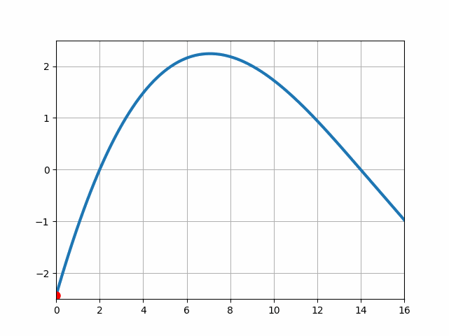
Starting with a short VBA sub-routine, using the Conbeam spreadsheet. The code simply generates a sequence of index numbers in a specified range, which are written to the spreadsheet, and the associated position of the applied point load is generated on the spreadsheet and passed to the ConBeam function that generates the required output, in this case the beam vertical deflections.

Sub Animate()
Dim Start As Long, Stp As Long, Target As Variant, EndPause As Double
Start = Range("U25").Value
Stp = Range("V25").Value

Set Target = Range("S25")
ActiveSheet.ChartObjects("Chart 1").Activate
' Enable screen updates for real-time visualization
Application.ScreenUpdating = True
    For i = Start To Stp
        Target.Value = i
        ActiveChart.Refresh
        
        EndPause = Timer + 0.05
        Do While Timer < EndPause
        ActiveSheet.Calculate
        DoEvents
        Loop
    Next
End Sub

The animation displays in Excel as an Excel chart object. To display as a GIF:

• Copy the active animation using a screen capture programme such as Snagit.
• Save as an MP4 file
• Convert to GIF with an on-line app, such as: MP4 to GIF Converter

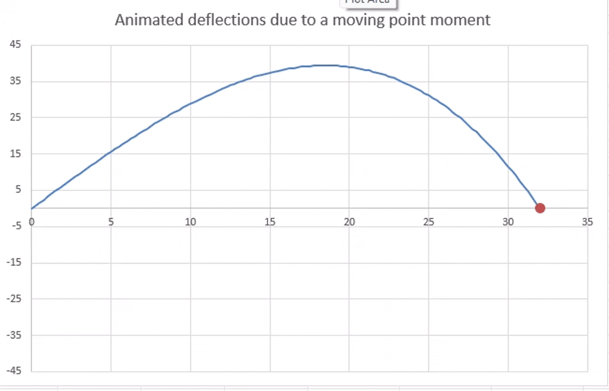
The first Python function generates a similar graph (deflections due to a moving point moment), using the py_ConBeam function, but with the following differences:

• The code is written as an Excel User Defined Function, using pyxll, with all input data included in the function input.
• The deflections are calculated using the py_ConBeam function, called from the Python Code.
• The animation is generated within the function using Matplotlib, and then written to the spreadsheet as a graphics object.
• Optionally, the animation can be written to a GIF file, which can then be used in any program accepting the GIF format, including the examples below.

Python code for the moving point load animation:

@xl_func
@xl_arg('Segments', 'numpy_array', ndim = 2) 
@xl_arg('Supports', 'numpy_array', ndim = 2) 
@xl_arg('DLoads', 'numpy_array', ndim = 2)
@xl_arg('PLoads', 'numpy_array', ndim = 2)
@xl_arg('replot', 'bool')
@xl_arg('miny', 'float')
@xl_arg('maxy', 'float')
@xl_arg('savegif', 'bool')
def plot_momdef(Segments, Supports, DLoads, PLoads, replot = False, miny=-4, maxy=4, savegif = False):
    Supports0 = np.copy(Supports)
    if replot:
        OutPoints=np.zeros((101,1))
        endx = Segments[-1,0]
        OutPoints[:,0] = np.linspace(0, endx, 101)
        # Create the matplotlib Figure object, axes and a line
        fig = plt.figure(facecolor='white')
        ax = plt.axes(xlim=(0, endx), ylim=(miny, maxy ))
        plt.grid(True)
        line, = ax.plot([], [], lw=3)
        point, = ax.plot([], [], 'ro', markersize=8)

        # The init function is called at the start of the animation
        def init():
            line.set_data([], [])
            point.set_data([], [])
            return line, point,
        i = 1
        # The animate function is called for each frame of the animation
        def animate(i):
            x = np.linspace(0, endx, 101)
            PLoads[0,0] = OutPoints[i]
            Supports = np.copy(Supports0)
            res = py_ConBeam(Segments, OutPoints, Supports, DLoads, PLoads,1,True)
            # convert y to mm
            y = res[:,4]*1000
            line.set_data(x, y)
            x2 = np.array([OutPoints[i]])
            y2 = np.array([y[i]])
            point.set_data(x2, y2)  
            return line, point, 
        
        # Construct the Animation object        
        anim = FuncAnimation(fig,
                            animate,
                            init_func=init,
                            frames=100,
                            interval=50,
                            blit=True)

        # Call pyxll.plot with the Animation object to render the animation
        # and display it in Excel.
        plot(anim, allow_resize=False)
        # Set savegif to True to save anaimation as a gif file
        if savegif: anim.save("pointmomdef.gif", writer=PillowWriter(fps=30))
    return 'Deflections for moving point moment'

Animation generated by the Python code above:

For this example 2 m long cantilevers were added at each end of the beam, and multi-span continuous beams are also possible.

The examples above generate animations for a single applied point moment, but the py_ConBeam spreadsheet includes a moving load function which allows a vehicle with any number of axles to be generated and applied to a continuous beam with any number of spans. The animations below have been generated using this function with a three span beam with short link slab spans at each support, and the M1600 vehicle from the Australian Bridge Design Code (AS 5100.2).

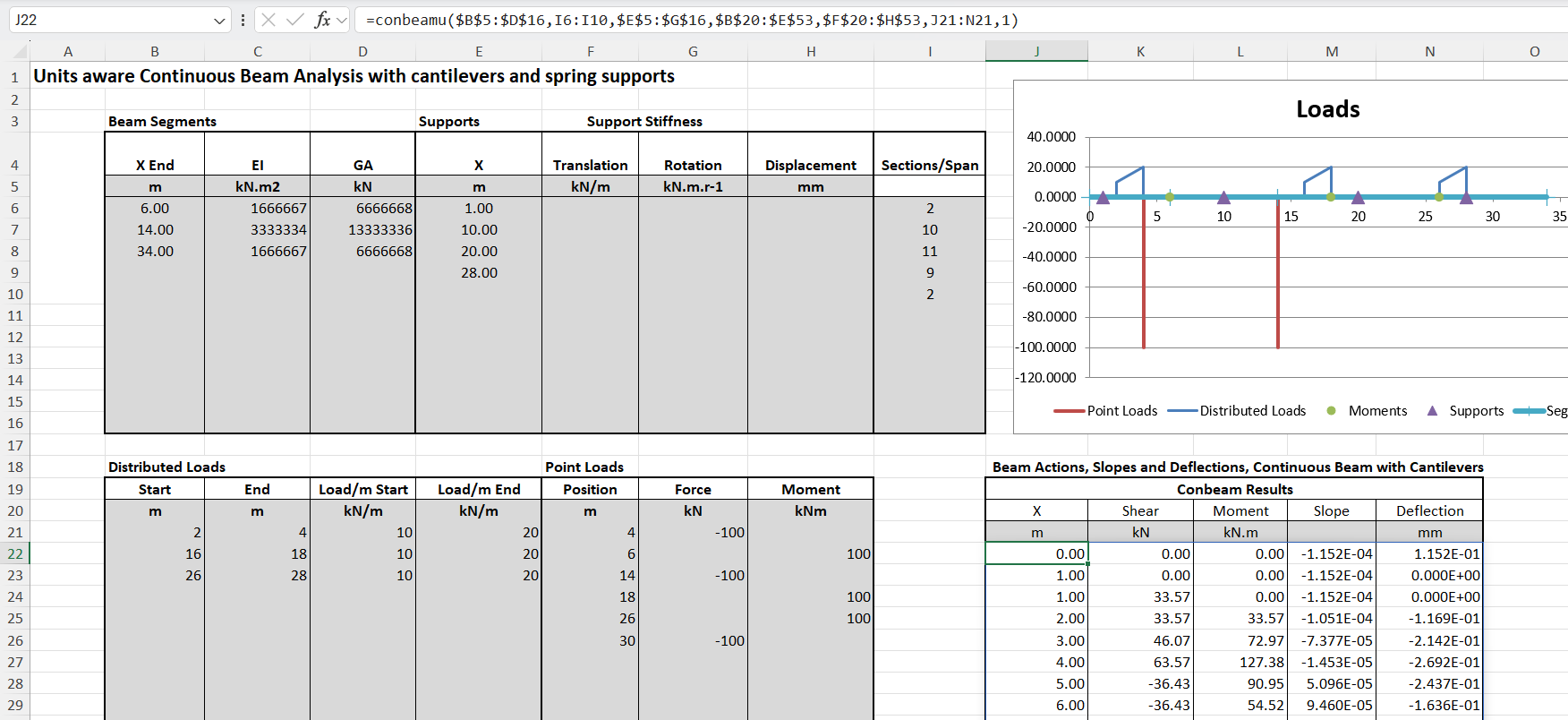
The beam segment lengths and cross section properties, and support locations and properties are defined in the usual way. Output points should be generated at equal spacing, and are defined by the number of sections per span:

The Vehicle Definition, Load Factors, and Output Units are defined as in the py_MovLoad function. The vehicle positions are defined with the starting and end point of the first axle, together with the number of positions. The graph options include:

• The action to be plotted; one of Shear, Moment, Slope or Deflection
• Option to re-plot the animation.
• Time interval between vehicle positions (milliseconds)
• Option to save the pot to a gif file.

Note that the plot generation process is quite slow, so the re-plot option should be turned off (0) except when the input has been changed.

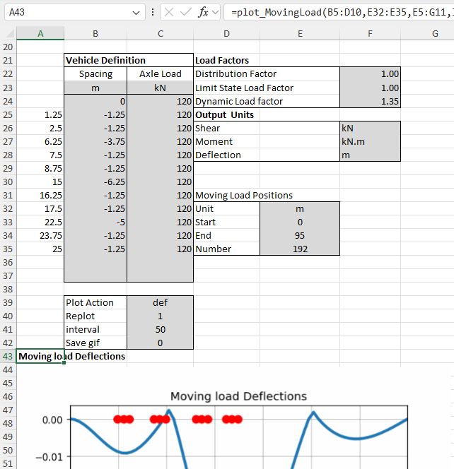
The moving load animation is generated immediately under the cell where the plot_MovingLoad function is entered:

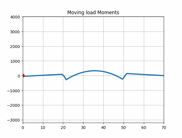
As mentioned above, the output options include:

Bending moment:

Shear force:

Slope:

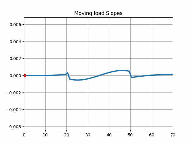
and deflection: