This post looks at alternative solutions to a problem posted on Quora:
One of the alternatives requires a new function linking to Scipy that has been added to the pyScipy module, that can be downloaded from:
For more details of the many functions linking Excel to Scipy (and related Python modules), through pyxll, see:
Scipy functions with Excel and pyxll and the following posts.
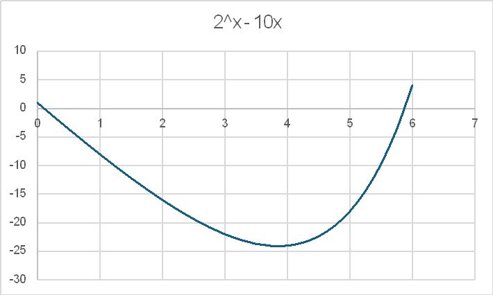
A quick plot of the function 2^x – 10x shows that there are solutions at x just greater than 0 and just less than 6:
The simplest and easiest way to get a close estimate of the exact solutions is to use the Excel Goal Seek function (although this wasn’t mentioned in any of the replies on Quora!). It is found under What-if Analysis on the Data tab:
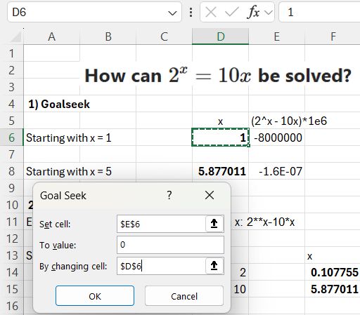
The required inputs are an initial guess of the ‘x’ value and the function to be solved. In this example, since we are looking for the x value to make the function zero, I have multiplied it by 1 million for greater precision. Goal Seek adjusts the value in cell D6 to make cell E6 very close to zero:
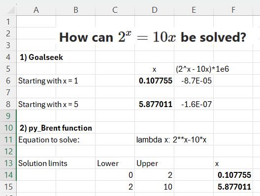
In this case starting with x = 1 returns a result of 0.107755, and x = 5 returns 5.877011.
The most frequent solution given in the Quora discussion was to use the Newton-Raphson method to find the two solutions by iteration. This can be done in Excel using the py_Brent function (which is a refinement of the Newton-Raphson method), that calls the Scipy brentq function, and is included in the Scipy download linked above. There is also a VBA version that can be downloaded from:
See Newton-Raphson and Brent’s Method – Solver examples for background information and examples.
The py_Brent function requires an input lower and upper bound for the solution, which must evaluate to values with different signs, and a text function in Python lambda format. Note that exponentiation must be in Python format (**), rather than ^.
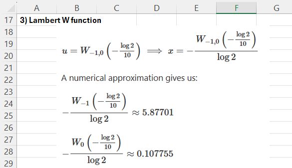
The third alternative is to use the Lambert W function, which is defined by W(z) = w, where we^w = z. The function has an infinite number of solutions with complex numbers, but for real results there are just two, indicated as W(0) and W(-1). See Lambert W function for more details.
The Lambert W function can be used to find the desired results as shown below:
Scipy has a lambertw function, that can be called from Excel using the pyScipy py_CallfuncS function:
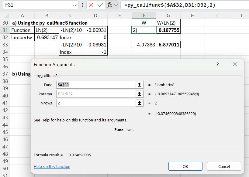
The required input is the function name (lambertw), the function input value and output index (0 or -1), entered in a column, and the number of input rows. The returned value is divided by LN(2) to find the required results.
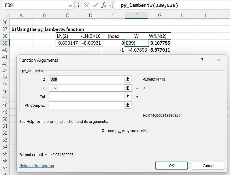
The py_CallfuncS function does not allow for input or output of complex numbers. To allow that, I have added the py_LambertW function to the pyScipy module, included in the download at the top of the post.
For the current example the input Z value is specified in a single cell, but complex numbers may be specified in two adjacent cells, or multiple complex numbers in a 2 column range. The function also allows adjustment of the target tolerance value, and the option to return complex numbers. By default results are returned as real for real input or complex for complex input, but the function result may be complex for real input with K other than 0 or -1, in which case RtnComplex should be set to True.
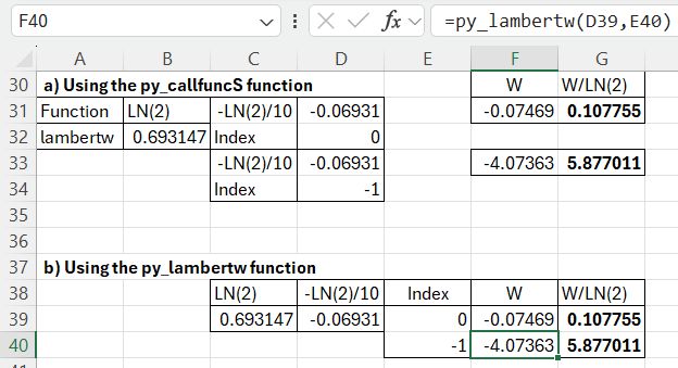
The final results using the LambertW functions are as for the other options:
The examples shown above can be downloaded from: Lambert.zip