Two new download sites with some of my favourite music from the 1960’s:
Bert at the BBC from bandcamp:
https://bertjansch.bandcamp.com/album/bert-at-the-bbc
… and for something completely different, assorted recordings from Tom Lehrer:

Two new download sites with some of my favourite music from the 1960’s:
Bert at the BBC from bandcamp:
https://bertjansch.bandcamp.com/album/bert-at-the-bbc
… and for something completely different, assorted recordings from Tom Lehrer:
I have now transferred the Ultimate Limit State design functions from the VBA RC Design Functions spreadsheet to Python format. The new spreadsheet and Python code can be downloaded from:
The code also includes the OptShearCap3600 function, described in the previous post.
The python code requires pyxll to connect to Excel. If this is installed, and “RC_UMom” is added to the list of modules to load at start-up in the pyxll.cfg file, the new functions should be available from any spreadsheet.
The included functions are:
py_UMom: ULS design of rectangular sections with two layers of reinforcement under combined bending, axial load, shear and torsion, to Australian and international codes. (Provision for prestressing will be added in the near future):

py_UmomPF: As above, but for Eurocode and British codes using a partial factor approach:

MaxAx: Maximum axial load for short or slender columns:

Devlength: Reinforcement development length to Australian, Eurocode, or British codes:

ShearCap3600: Shear capacity to current AS 3600 and 5100.5:
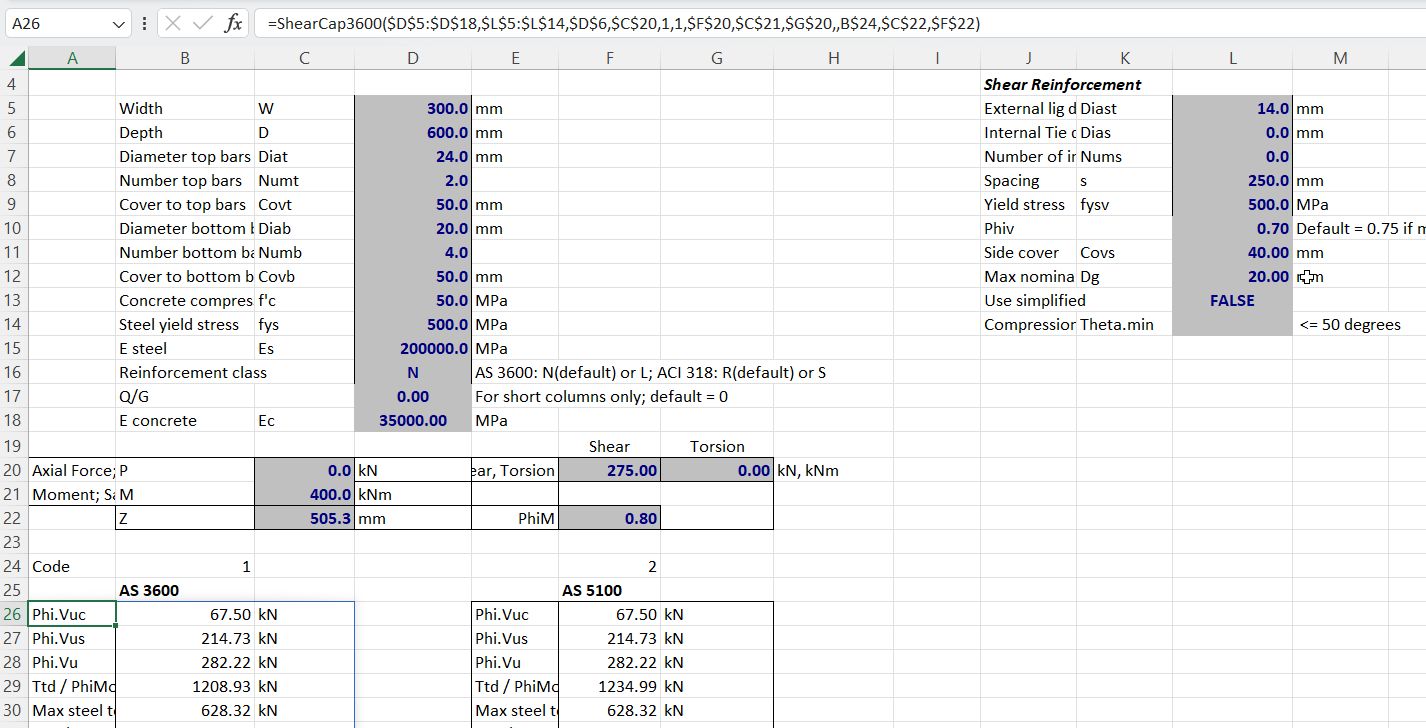
OptShearCap3600: Optimise shear capacity for given moment/shear ratio by adjusting the compression strut angle:

Extracts of the OptShearCap3600 function code are shown below. The scipy.optimize.brentq function is used to adjust the applied loads to be equal to the design section capacity:
# create list of arguments for the py_Umom function, called by the Scipy brentq function
    args = [InCells, Puin, 13, 1, Muin, [] , ShearReo, Code, VTuin]

    # Use scipy.optimize.brentq to adjust the input shear force to be equal to the design capacity
    try:
        res  = sopt.brentq(call_Umom, mincap, maxcap, args = args, maxiter = 100)
    except:
        outA[0,0] = 1
        return outA

# The call_Umom function adjusts the input loads in proportion to the shear force
#  passed by brentq, then calls py_Umom and returns the difference between the
#  applied shear and shear capacity

def call_Umom(Vstar, args):
    args[8][0,0] = Vstar
    args[4][0] = Vstar * MoV
    if ToV != 0: args[8][0,1] = Vstar * ToV
    if PoV != 0: args[1][0] = Vstar * PoV
    res = py_Umom(*args )
    return res[1]
Similar procedures are used to adjust the applied moment when this is critical, or the compression strut angle in the intermediate range, so that both shear and moment capacities are equal to the applied actions.
Further to the last post on this subject I have been looking at procedures to speed up design for shear to AS 3600 when the “refined” analysis procedure is used. The issues that need to be addressed are:
I have now written a Python function to carry out the iterations using the Scipy brentq function with the procedure outlined below:
Typical function output is shown in the screenshot below:
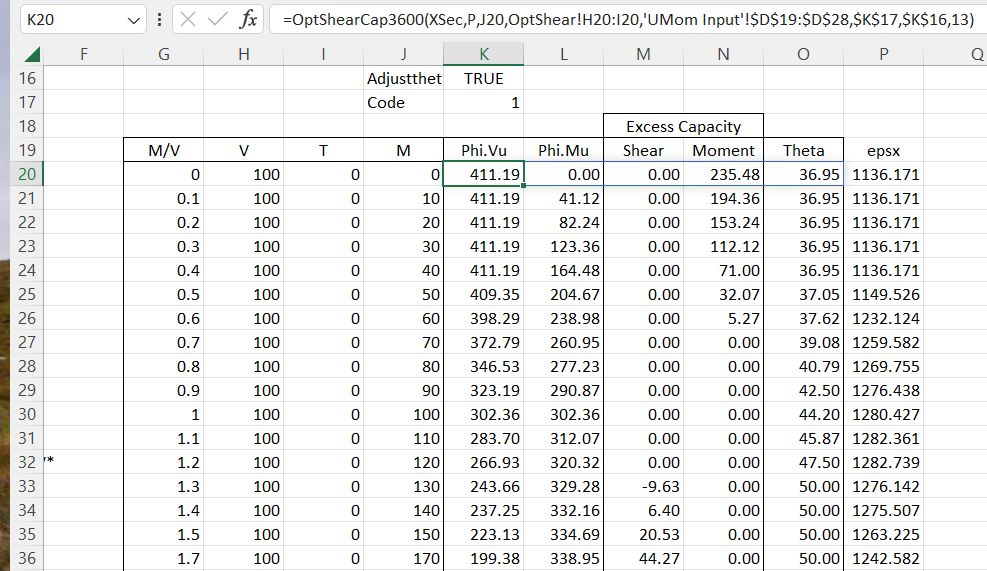
In this example the section has been analysed for a constant shear force with an increasing M/V ratio. The function output (Columns K to O) is:
These results are plotted below with typical shear and bending loads, taken from a heavy road vehicle travelling over an 8 metre simply supported span, with the loads plotted at 0.4 and 1.0 metres from the support. The capacity is also plotted with no adjustment of the compression strut angle, showing a significantly reduced capacity.
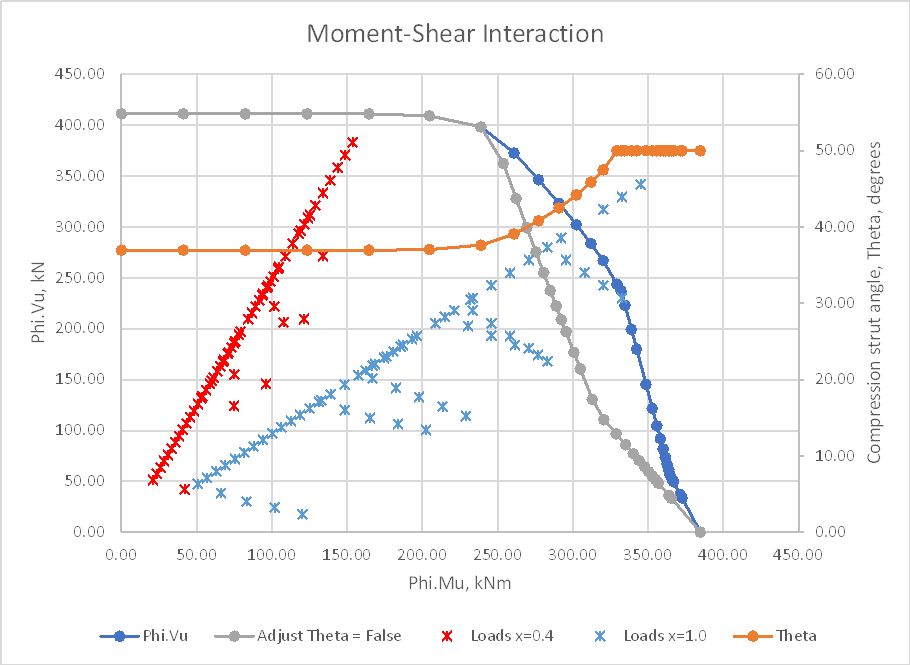
Plotting the section capacity as a moment-shear interaction diagram allows the loads from all sections with identical reinforcement to be plotted on the same section, and load cases where the applied loads exceed the section capacity are immediately visible.
This is a work in progress, but a spreadsheet with all necessary Python files will be available for download shortly.
There have been many posts here looking at alternative ways of working with functions entered as text on a spreadsheet, and working with units, most recently here.
One drawback with this approach is that text in an Excel cell must be ASCII or Unicode, which has limited capabilities for presenting maths text in a readable form. Excel does allow elaborate maths equations to be generated and displayed, but as far as I know there is no way to interact with these equations from VBA, so they can neither be generated by code, or evaluated by code.
Python on the other hand has libraries that will convert plain text equations to Latex (and other formats), and display Latex code. I have now written a Python function “plot_math” using a combination of Sympy, Pint, and Matplotlib to:
The new code can be downloaded from:
The spreadsheet requires the following software:
The download file includes two Python files:
Startup_min.py includes the plot_math function, and should be added to the list of files to open at start-up in pyxll.cfg.
Note that this is a work in progress. If you have any problems with installation or running the programs, please let me know.
Some examples of the new function in action are shown below:
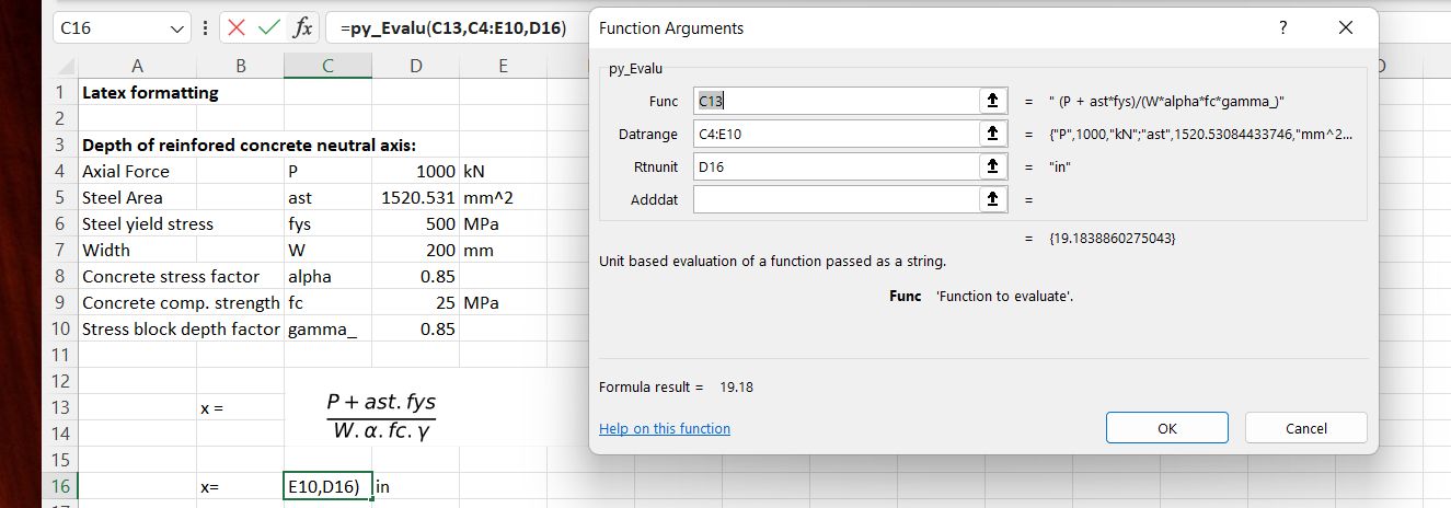
The text to be displayed (and optionally evaluated) should be entered as plain text at any chosen location. In the example below the plot_math function is then entered in the cell immediately above (C12).

When the plot_math function is entered the image will display immediately below:

The image can then be dragged to the desired location; in this case so that the original text and the function return value (0) are hidden. In this example the numerical value of the function for selected input values is displayed using the py_Evalu function.
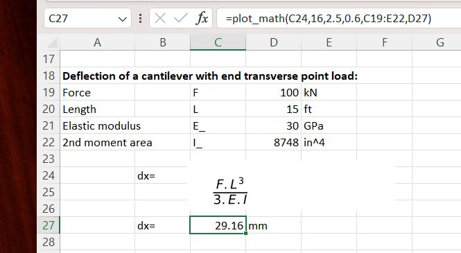
Alternatively the plot_math function will return the value of the function if suitable input data is selected:

In this case a three column data range has been selected, and also an output unit, so the calculation will be unit aware:

As before, the image is displayed immediately below the plot_math input cell, but can be dragged to any desired location:
Some other features to note:
We haven’t had any Bach for a bit, so here is:
An excellent cover of Anne Briggs’ song, Go Your Way:
And Anne Briggs herself singing the song, accompanied by Bert Jansch:
And another cover (posted here 12 years ago yesterday):
