Jack Orion

This is what Wikipedia says of the music played by The Pentangle:

Pentangle are usually characterised as a folk-rock band. Danny Thompson preferred to describe the group as a “folk-jazz band.”[25] John Renbourn also rejected the “folk-rock” categorisation, saying, “One of the worst things you can do to a folk song is inflict a rock beat on it. . . Most of the old songs that I have heard have their own internal rhythm. When we worked on those in the group, Terry Cox worked out his percussion patterns to match the patterns in the songs exactly. In that respect he was the opposite of a folk-rock drummer.”[26] This approach to songs led to the use of unusual time signatures: “Market Song” from Sweet Child moves from 7/4 to 11/4 and 4/4 time,[27] and “Light Flight” from Basket of Light includes sections in 5/8, 7/8 and 6/4.[28]

Writing in The Times,Henry Raynor struggled to characterise their music: “It is not a pop group, not a folk group and not a jazz group, but what it attempts is music which is a synthesis of all these and other styles as well as interesting experiments in each of them individually.”

There is no better example of their unique style than their version of “Jack Orion” on their 1970 album “Cruel Sister”, and I have just discovered an uninterrupted recording of the full 18 minute song on You Tube:

Posted in Bach | Tagged , | Leave a comment

Frame Analysis with Excel

Starting from 2009 I have posted a series on frame analysis using Excel, starting from a simple “on-sheet” solution and working through to applications able to solve large 2D or 3D problems. To follow the analysis process it is best to read these posts in sequence, but the links between them are hidden in the comments, and in one case the link seems to be missing, so here is a list of all the frame analysis related posts, in date order:

This covers all the posts here directly related to the frame analysis spreadsheets.  There are also many related posts covering analysis of continuous beams, and on-going work on linking the frame analysis spreadsheets to Python based solver routines, and these may be found by selecting Frame Analysis in the Categories drop-down box in the top-right corner.

Posted in Excel, Frame Analysis, VBA | Tagged , , , | 1 Comment

Two MaxAbs functions

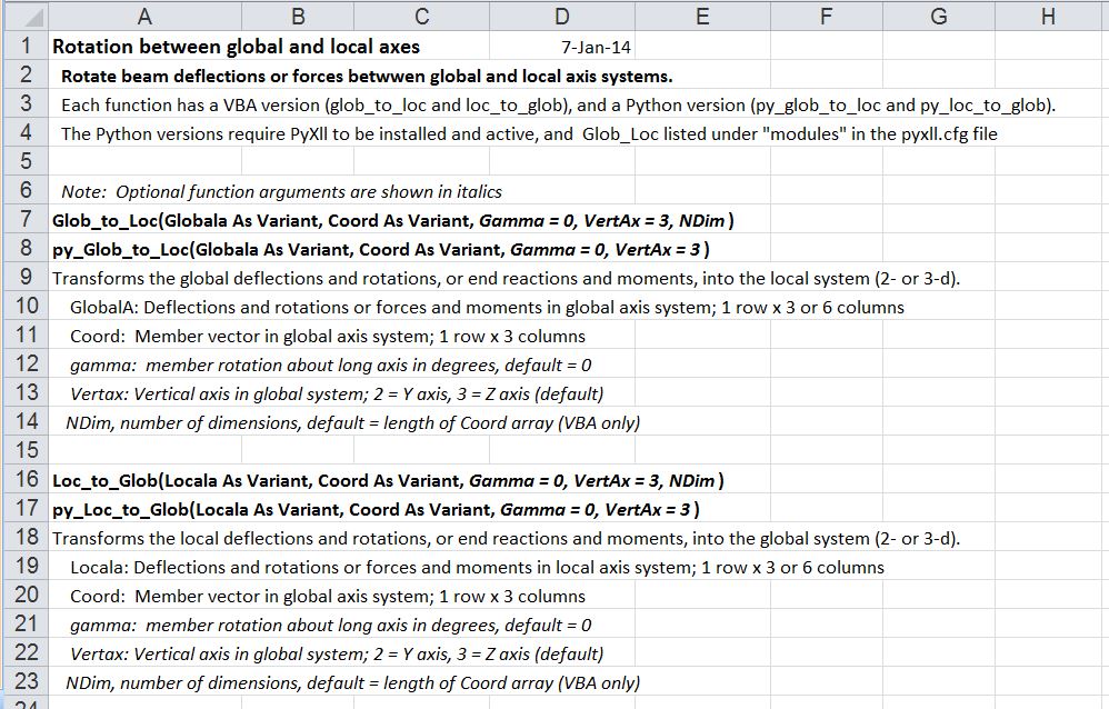
Excel does not have a built-in function to find the maximum absolute value of a range, perhaps because the Max() and Abs() functions can be combined in an array function:

  • =Max(Abs(datarange))

This solution has a number of drawbacks however:

  • The function must be entered as an array function, by pressing Ctrl-Shift-Enter, rather than just enter.
  • If it is entered with just pressing the Enter key it displays the wrong value, rather than an error message.
  • Even if it is entered correctly, if anyone presses F2 then enter it will revert to a normal function, and display the wrong result.
  • It is not available from VBA.

For all these reasons I decided to write a MaxAbs function in VBA, that can be called either from the worksheet, or from another VBA routine.  Here is the code, Version 1:

Function MaxAbs(Dataa As Variant) As Double
Dim MaxVal As Double, Val As Variant

    If TypeName(Dataa) = "Range" Then Dataa = Dataa.Value2

    For Each Val In Dataa
        If Abs(Val) > MaxVal Then MaxVal = Abs(Val)
    Next Val

    MaxAbs = MaxVal

End Function

Having done that, I wondered if calling the built-in Max function might work better, particularly for big data ranges. My first effort was:

Function MaxAbs2(Dataa As Variant) As Double
Dim MaxVal1 As Double, MaxVal2 As Double

    If TypeName(Dataa) = "Range" Then Dataa = Dataa.Value2

    MaxVal1 = WorksheetFunction.Max(Dataa)
    MaxVal2 = -WorksheetFunction.Min(Dataa)

    If MaxVal1 > MaxVal2 Then MaxAbs2 = MaxVal1 Else MaxAbs2 = MaxVal2

End Function

This proved to be slower than the first version, even for very big data ranges, but working with ranges rather than variant arrays:

Function MaxAbsR(Dataa As Range) As Double
Dim MaxVal1 As Double, MaxVal2 As Double
    MaxVal1 = WorksheetFunction.Max(Dataa)
    MaxVal2 = -WorksheetFunction.Min(Dataa)

    If MaxVal1 > MaxVal2 Then MaxAbsR = MaxVal1 Else MaxAbsR = MaxVal2

End Function

made the code faster than the original version for anything more than about 15 rows. The drawback with this version is that if you are working with double or variant arrays in VBA (which I usually am), these would need to be converted to range objects first, so I ended up with the two versions:

  • MaxAbs() for use with arrays in VBA
  • MaxAbsR() for use as a UDF on the spreadsheet, or on range objects in VBA

The first function can also be easily adapted to provide the minimum absolute value:

Function MinAbs(Dataa As Variant) As Double
Dim MinVal As Double, Val As Variant

    If TypeName(Dataa) = "Range" Then Dataa = Dataa.Value2
    MinVal = 1E+308
    For Each Val In Dataa
        If Abs(Val) < MinVal Then MinVal = Abs(Val)
    Next Val

    MinAbs = MinVal

End Function

Other than changing max to min, and > to <, the only difference is that MinVal is set to a very large number before starting the loop; otherwise it would always return zero.

Posted in Arrays, Excel, Maths, Newton, UDFs, VBA | Tagged , , , , | 9 Comments

Solving Quadratic, Cubic, Quartic and higher order equations; examples

A previous post presented a spreadsheet with functions for solving cubic and quartic equations, and this has been extended with another function solving higher order polynomials.  The functions are actually very easy to use, but the documentation in the spreadsheets is quite brief, and the large number of options presented may be off-putting.

To make these functions more accessible, this post presents an example of using the cubic function, and some notes on alternatives and usage of the other functions.  These examples have been added as a separate file to the download file : Polynomial.zip.  As usual, the download files include full open-source code.  Those interested in the included Python functions, see: Python for VBA users – 5; Using built in numpy functions.

The problem to be solved is, if we have a cubic polynomial equation of the form:
Y = aX^3 + bX^2 + cX + e
how do we find the value or values of X that satisfy this equation for known values of a, b, c, and e, and any given Y?

The procedure is:

  • Rearrange the equation to the form:
    aX^3 + bX^2 + cX + d = 0
    by subtracting Y from both sides; that is: d = e – Y.
  • Enter the coefficients, a to d, in a single column or row:
    polyroots2-1
  • Enter the cubic function, with the range of coefficient values as the argument.
  • This will return one of the three solutions to the cubic equation.  To display all three solutions, plus the number of real solutions, enter as an array function:
    –  Select the cell containing the function, and the three cells below.
    – Press the F2 key (Edit)
    – Press Ctrl-Shift-Enter
    The four required values will be displayed as shown below:

polyroots2-2
This is a plot of the cubic function solved.  It can be seen that the three solutions are the X values where the function is equal to zero.
polyroots2-3
Some cubic equations, such as in the graph below, have only one “real” solution, and two “complex” solutions, i.e. solutions with a “real” and “imaginary” part.
polyroots2-5
If the complex solutions are required the CubicC function must be used.  This function is used in the same way as Cubic, except that the output range is two columns; for the real and imaginary parts of the solution:
polyroots2-4
If it is desired to display a single solution, other than the first, this can be done with the optional Out1, and Out2 arguments, as shown below.  Alternatively the built-in Excel Index function may be used.
polyroots2-6
The functions Quadratic and Quartic operate in the same way as Cubic, except that they will also return complex results, so no QuadraticC or QuarticC functions are required.

The function RPolyJT may be used as an alternative to Quadratic, Cubic and Quartic, and also for higher order polynomials.  RPolyJT uses the Jenkins-Traub iterative solution, and is a little slower than the other functions, but will return results nearly instantaneously in most circumstances, and can sometimes be more accurate than the other functions.
polyroots2-7

Further notes and examples are given in the download file. If anything remains unclear, please ask.

Posted in Arrays, Excel, Link to Python, Maths, Newton, UDFs, VBA | Tagged , , , , , , , , , | 13 Comments

Converting from global to local coordinates (and vice versa)

In 3D structural analysis (as well as many other applications) it is necessary to convert section properties, forces, and deflections between coordinate systems defined by individual structural members (local coordinates) and the common coordinate system defining the entire structure (global coordinates).  For a 2D analysis this is straightforward, but for 3D analysis the transformation needs to be carefully defined to avoid unexpected results.  Functions to perform this operation are included in the 3D frame analysis presented here previously (most recently here), but since these functions have other applications I have extracted them and added them to the IP2 spreadsheet.

Download IP2.zip with full open source code.

The new functions are glob_to_loc() and loc_to_glob, which also come in Python versions (py_glob_to_loc() and py_loc_to_glob).  Use of the Python versions requires the PyXll add-in.  See Installing Python, Scipy and Pyxll for more details. Details of usage are shown in the screen-shot below (also included in the download file).:

glob_loc1

glob_to_loc and loc_to_glob functions (click for full size view)

The function arguments are:

  • Globala or Locala: the values to be converted to the new axis system.  The values may be deflections, rotations, forces, bending moments, or section properties (translational and rotational stiffness values).  The Globala and Locala arrays may contain 3 or 6 elements; for instance deflections in the X, Y and Z directions, followed by rotations associated with those deflections.  Global values are always listed in the order X, Y, Z.  See below for the definition and order of the local axes.
  • Coord: a 3 element array defining the direction of the longitudinal local axis, relative to the global axis system.  In the context of a frame analysis it is the length of the beam element in the X, Y and Z directions.
  • Gamma: an angle (in degrees) defining the orientation of the local axes, relative to the default alignment (see below).
  • Vertax: 2 or 3, the default vertical direction of the local axes.  This value defines both the vertical direction and the ordering of the local axes (see below).

There are a number of options for defining the default orientation and numbering of the local axes; the two I have chosen are:

  • Vertax = 2:  Local Axis 1 is aligned with the longitudinal axis of the beam, from node 1 to node 2.  Axis 2 is perpendicular to Axis 1 and parallel to the X-Z plane, so the Y axis is in effect treated as vertical.  Axis 3 completes the orthogonal system, being perpendicular to both Axis 1 and Axis 2.  This is the system used in the book “Programming the Finite Element Method”, which is the source of many of the routines used in the frame analysis spreadsheets.
  • Vertax = 3: Local Axis 3 is aligned with the longitudinal axis of the beam, from node 1 to node 2.  Axis 2 is perpendicular to Axis 3 and parallel to the X-Y plane, so the Z axis is treated as vertical.  Axis 1 completes the orthogonal system, being perpendicular to both Axis 3 and Axis 2.  This is the system used in the program Strand7, which I have used to check the results of my spreadsheets.

The screen-shot below shows the results of generating four I-beams in Strand7, using the default local axis system:

glob_loc0

Note that Axis 2 for all four beams is parallel to the XY Plane.  Also note that by default the web of the I beams is also aligned with Axis 2.

The next screen-shot shows the result of rotating the view of the model, so that the Y axis is vertical, rather than the Z axis:

glob_loc0a

Now the webs of the horizontal members are vertical, but note that the web of the inclined member is now inclined.

The simplest way to achieve a vertical web orientation in all members is to use the Z axis as the vertical direction, and rotate the principal axes of all the beams through 90 degrees, as shown below:
glob_loc0b

The two screen-shots below show the results of the glob_to_loc function for  beam aligned with the X axis, and with Vertax set to 2 and 3 respectively.  The results are the same except that Local Axes 1 and 3 are swapped and the sign of the Axis 3/1 values has changed.  Note that applying loc_to_glob with the appropriate Vertax value returns the original data.
glob_loc2a

glob_loc2b
Similar results are seen for a beam lying in the XY plane:
glob_loc3
The sign of the Axis 3/1 values can be changed by applying a rotation of 90 degrees:
glob_loc4
For an inclined beam the changing the Vertax value leaves the axial results unchanged (Axis 1/3), but the other axes have differing results, due to the differing rotations of the beams.  The function results are compared with results from Strand7, showing exact agreement:
glob_loc5
The results of the different Vertax options may be equalised by applying a rotation to one of the beams, bringing the beam principal axes back into alignment:
glob_loc6

Posted in Excel, Finite Element Analysis, Frame Analysis, Link to Python, Maths, UDFs, VBA | Tagged , , , , , , , | 22 Comments