As in previous years, I have downloaded the statistics for this blog for the previous year, and pasted them into a worksheet. The link to each post is preserved in the spreadsheet, so it makes a convenient index to what has been posted over the year. The spreadsheet has been uploaded to Skydrive (which now seems to have morphed into OneDrive), so you should be able to access the links in the window below, or open the file in your browser or Excel, or download it.
Of the 2013 posts, the most popular overall was Clearing excess formats .
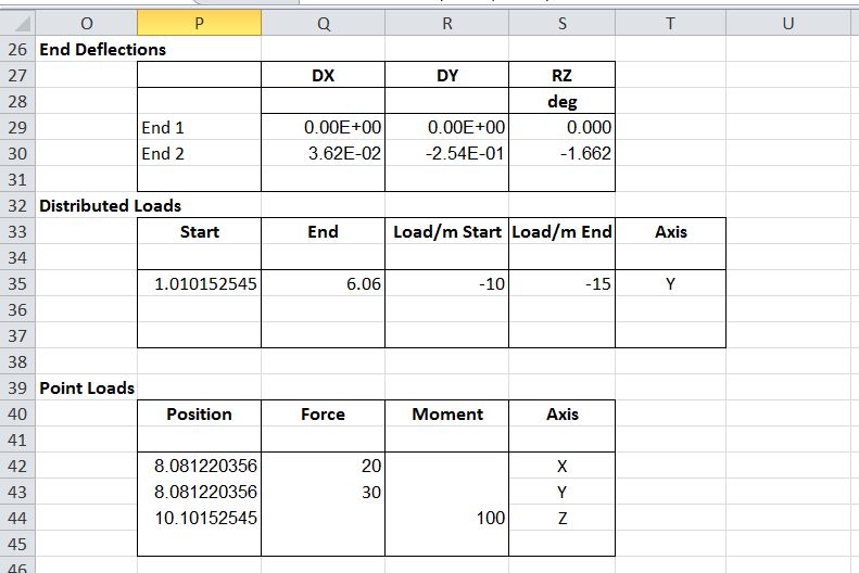
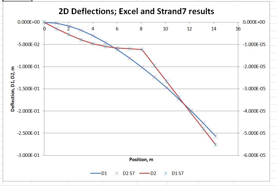
The most popular in the Newton category was 3DFrame – 3D Frame analysis for Excel,
and the most popular in the Bach category (by a mile) was George Gently, Matty Groves, and Ebony Buckle
From the “deserving but sadly neglected category” I have chosen (so go and have a look/listen):
Newton: Unit aware continuous beam spreadsheet update
Excel: Selecting Ranges from a UDF:
Bach: The Incredible String Band
Most frequent referrers to this site came from:
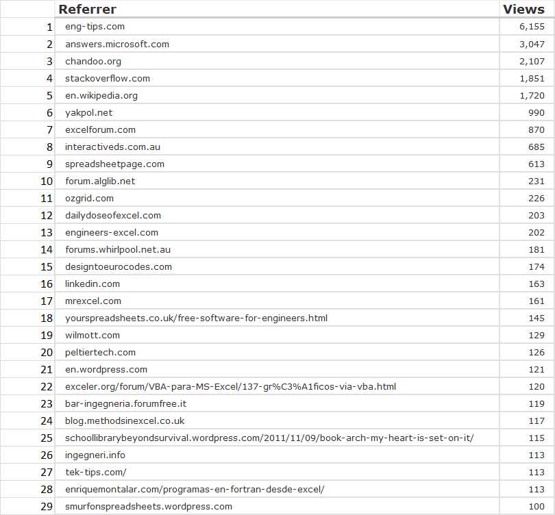
Referrers to NewtonExcelBach