Reinforced Concrete Section Analysis – 5; Ultimate Limit State

Previous posts in this series have looked at the analysis of beams where the steel stress is within the elastic range, and the concrete stress is sufficiently low that the assumption of linear elastic behaviour in compression is a reasonable approximation.  I now move on to analysis for the ultimate limit state, where some or all of the steel is past its yield stress, and the concrete compression zone may be analysed as having a constant stress, close to its failure stress.

The file ULS Design Functions.zip contains User Defined Functions (UDF’s) that will find the ultimate bending capacity of any reinforced or prestressed concrete section (defined by rectangular or trapezoidal layers) with any number of layers of reinforcement, when subject to a specified axial load.  As for the elastic design functions, the analysis uses a closed form solution, rather than an iterative procedure.  The current version follows the Australian Standards AS 3600 or AS 5100.  Other codes will be added to future versions. Details of the procedure will be given in later posts.

Screen shots:

Input, circular section

Input, circular section

Output, circular section

Output, circular section

Interaction diagram

Interaction diagram

Posted in Beam Bending, Excel, UDFs | Tagged , , , , , , , | 5 Comments

Back to Bassics

Browsing John Walkenbach’s non-Excel blog : The J-Walk Blog  reminded me that Bach hasn’t had a look in here recently, so here is a clip of one of my all time favourite musicians, Danny Thompson (playing here with John Martyn).  Plug in headphones or some decent external speakers to do it justice.

The Official Danny Thompson Web Site

Posted in Bach | Tagged , , | Leave a comment

Intersections, interpolations, and rotations

Amongst the many and varied functions provided by Excel (or as far as I know any other spreadsheet) there are none that provide a one step process for linear interpolation, finding the intersection points of lines, or conversion between polar and rectangular coordinates, and related operations.

These functions and more can be found in the spreadsheet:  IP.zip which includes open source code for the following functions:

Update 29th March 2011:  For the latest version of this spreadsheet, including many additional functions download IP2.zip.  See also the latest related blog post.

Intersection Functions
IP
Finds the intersection points of two 2D lines or polylines
=ip(Line1,LINE2,Optional Coordinate, Optional Point no)
“Line1” and “Line 2” are ranges listing the XY coordinates for the two lines
“Coordinate” specifies the ordinate required, 1 = X, 2 = Y
“Point No” specifies which intersection point is required
If “Point No” is not provided IP returns an n x 2 array, where n is the number of intersection points.
If “Coordinate” is not provided IP returns a 1 x 2 array if “Point no” is provided, or an n x 2 array if not.
If “Line2” is a single point IP returns intersection points for a line through this point and parallel to the X axis if XY = 1, or the Y axis if XY = 2

Intersection points of two polylines

Intersection points of two polylines

INSIDE
Finds if a specified point is inside a closed polyline
=INSIDE(Polyline, Point)

IPLC
Finds the intersection points of a 2D line and a circle
=IPLC(Line, CircleXY ,Radius)

IPCC
Finds the intersection points of two circles
=IPCC(Circle1XY, Radius1, Circle2XY, Radius2)

IPSSS, IPSS
IPSSS finds the 3D intersection points of three spheres
IPSS finds the location and radius of the intersection circle of two spheres,
and the polar coordinate angles of the line connecting the two cenrtres
=IPSSS(Sphere1XYZR, Sphere2XYZR, Sphere3XYZR)

=IPSS(Sphere1XYZR, Sphere2XYZR)
Distance from centre sphere1 to centre intersection circle, radius intersection circle,
and angle of line connecting sphere centres in XY plane and perpendicular plane (radians)

Rectangular to Polar Functions
RtoP, PtoR
Converts rectangular to polar coordinates and polar to rectangular
=RtoP(Rectangular Coordinate range, Origin, Coordinate number)
=PtoR(Polar Coordinate range, Origin, Coordinate number)
Coordinate number 1 2 3
Rectangular X Y Z
Polar R Theta1 Theta2
Theta1 = angle in XY plane
Theta2 = angle in perpendicular plane

Where an origin is given the origin is moved to the coordinates specified

Rotate
Rotates 2D or 3D rectangular axes about any axis
Rotate(Rectangular Coordinate range, Rotation in radians, Axis, Optional Coordinate Number)

Interploation Functions
interp =interp(tablerange, value, column no) Linear interpolation
interp2 =interp2(tablerange, row value, column val) 2 way linear interpolation
loginterp =loginterp(tablerange, value, column no) Log interpolation
loginterp2 =loginterp2(tablerange, row value, column val) 2 way log interpolation
quadinterp =quadinterp(tablerange, value, column no) Quadratic interpolation

Interpolation functions

Interpolation functions

Posted in Coordinate Geometry, Excel, UDFs, VBA | Tagged , , , , , , | 37 Comments

Ideas for suspension bridges

here: – mollwollfumble’s science

Some old, some new, some might work, some just plain weird.

Posted in Newton | Tagged | Leave a comment

Drawing in Excel 5 – Shape List

Previous Post

For some reason best known to Microsoft, the Excel documentation does not include a graphic list of shapes with an example of each shape, and the text list they do provide is incomplete. 

The file shapelist.zip

rectifies that omission with an automatically generated table of shapes from number 1 through to 183.

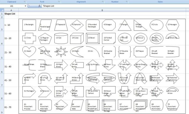
It also includes examples of how arcs (shape no. 25) work in Excel 2007 and earlier versions.
 

The size and position of arcs are defined with the usual width, height, left, and top properties, but note that the width and height are equal to the arc radius, and the left coordinate is equal to the X value of the arc centre.  The start and end points of the arc are defined with Adjustment(1) and Adjustment(2), and the shape thus defined may be rotated with the Rotation property.  Unfortunately there are significant differences in the way in which these properties are applied in Excel 2007 and earlier versions.

Assuming  an XY coordinate system, with origin at the centre of the arc:

Adjustment(1)  defines the angle of the start of the arc, measured from the X axis.  In Excel 2007 clockwise angles are positive, in earlier versions anti-clockwise is positive.

In both versions an Adjustment(1) value of zero defaults to a starting point on the Y axis, i.e. to -90 degrees in Excel 2007 and 90 degrees in earlier versions.

Adjustment(2) defines the angle of the end of the arc, measured from the X axis, with the same sign convention as adjustment(1).  An adjustment(2) value of zero defines an end point on the X axis, as would be expected, zero values for both adjustments therefore defines an arc between the Y and X axes.

The rotate property rotates the defined shape, with a clockwise rotation being positive in all Excel versions.

In Excel 2007 the shape is rotated about the origin, i.e. the centre of curvature of the arc.  In earlier versions the rotation appears to be about the mid-point of a radial line to the centre of the arc.

For compatibility between versions it seems best to avoid using the Rotation property, and adjust the sign of the adjustment angles according to the version number.

Code to generate an arc and a circle, using values specified in a spreadsheet range, is shown below.  The code checks for the Excel version, and for versions earlier than 2007 (version 12.0) reverses the sign of the arc adjustments, so that the arcs drawn are consistent across versions.

Sub Drawshape()

Dim shapeA As Variant, sType As MsoAutoShapeType, sLeft As Single, s_Top As Single, sWidth As Single

Dim sHeight As Single, sRotn As Single, sAdj1 As Single, sAdj2 As Single

Dim shp As Shape, i As Long

For Each shp In ActiveSheet.Shapes

shp.Delete

Next shp

shapeA = Range("shapetab").Value2

i = 1

Do While shapeA(1, i) <> 0

sType = shapeA(1, i)

sLeft = shapeA(2, i)

s_Top = shapeA(3, i)

sWidth = shapeA(4, i)

sHeight = shapeA(5, i)

sRotn = shapeA(6, i)

sAdj1 = shapeA(7, i)

sAdj2 = shapeA(8, i)

If Application.Version < 12 Then

sAdj1 = -sAdj1

sAdj2 = -sAdj2

End If

With ActiveSheet.Shapes

Set shp = .AddShape(sType, sLeft, s_Top, sWidth, sHeight)

End With

With shp

.Rotation = sRotn

If sAdj1 <> 0 Then .Adjustments(1) = sAdj1

If sAdj1 <> 0 Then .Adjustments(2) = sAdj2

.Fill.Visible = msoFalse

End With

i = i + 1

Loop

End Sub
 
An example of the shapes generated by this code is shown below:

Note that “Width” and “Height” values of the circle are double that of the arc, and the “Left” value of the circle is 105 less than that of the arc.


Use of the “rotation” property in Excel 2007 and earlier versions is illustrated below:


Note that the input for these two screen shots was identical.

Posted in Drawing, Excel, VBA | Tagged , , , | 4 Comments