Some thoughts on Magic …

… from Alana Hicks, Leonard Cohen, and Buffy St Marie.

Alana Hicks is a friend of my daughter’s.  This is her story:

smoke-and-fire

… which reminded me of a song I heard once on the radio over 40 years ago, and I have always remembered. Words by Leonard Cohen, sung by Buffy St Marie:


Posted in Bach | Tagged , , , , , | 2 Comments

The Conjugate Beam Method

The Conjugate Beam Method is a variation of the Moment-Area Method that allows beam slopes and deflections to be calculated purely from the calculation of shear forces and bending moments of the beam with (in some cases) modified support conditions.  Both methods were developed by Christian Otto Mohr, although the Conjugate Beam Method is often attributed to others.  I will have a closer look at the history in a later post, but in this post I will look at how it works, with a simple Excel based example.

The basis of the method is:

  1. Calculate the bending moment diagram for the real beam with the actual support conditions.
  2. Apply the bending moment diagram divided by EI to the “conjugate beam”,  as a distributed load.  The conjugate beam is an imaginary beam of the same length, with support conditions modified as described below. (E = elastic modulus; I = second moment of area.  Note that both may vary along the length of the beam).
  3. Calculate the shear force and bending moment diagram for the conjugate beam.  At any cross section the numerical value of the shear force is then equal to the slope of the real beam, and the bending moment is equal to the deflection of the real beam.

The changes to the support conditions in the conjugate beam are based on the following requirements:

  • At any point where the deflection is zero the conjugate beam moment must be zero, requiring either a simple end support or free end, or an internal hinge.
  • Where the end slope is zero the conjugate beam shear must be zero, requiring a free end.
  • Similarly, where the deflection or slope is non-zero the conjugate beam must be able to generate a moment or shear force.
  • Where there is a discontinuity in the slope (at an internal hinge) the conjugate beam must have a simple support.

These modifications to the support conditions are illustrated below (from the Wikipedia Article):

conjugate1-0

The spreadsheet ConjugateBeam.zip provides a simple example of the method applied to a simply supported beam with two point loads:

conjugate1-1

The shear and moment diagrams are calculated for the specified load positions and values, using the usual methods (Columns B and C above):

conjugate1-2

The bending moment due to the applied load is then divided by EI to give the applied load for the conjugate beam.  For a simply supported beam the conjugate beam supports are unchanged, but we need to calculate the reaction force at the supports.  A convenient way to do that is to treat the conjugate beam as a cantilever fixed at End 2, and calculate the shear and moment at End 2 (Columns E and F).  The End 1 shear force for the simply supported beam is then minus this moment, divided by the beam length, and this force is applied along the full length of the beam(Column G and below):

conjugate1-3

The conjugate beam bending moment diagram is now found for the simply supported shear diagram (Column H and below):

conjugate1-4

Note that the bending moment at End 2 is exactly zero, as would be expected.  The numerical values of the conjugate beam shear and bending moment are equal to the slope and displacement of the original beam.

An alternative calculation of the shear force at End 1 of the conjugate beam is shown below; taking moments about End 1, to find the reaction at End 2, and hence the End 1 force.  In both cases the calculation is equivalent to calculating the deflection at the end of a cantilever, and dividing by the beam length to find the rotation required to return the beam to horizontal.

conjugate1-5

In general the maximum deflection of the beam will be intermediate between the two applied loads.  The Excel solver has been set up in the spreadsheet to find this location by adjusting the value in cell A18 so that the conjugate beam shear (equal to the original beam slope) is equal to zero.  This is the point of maximum bending moment in the conjugate beam, and maximum deflection in the original beam:

conjugate1-6

To run the solver, select the Data tab, click the solver icon (extreme right), then click solve.  If the solver icon does not display the solver must be installed from the File-Options-Add ins menu.

Posted in Beam Bending, Excel, Frame Analysis, Newton | Tagged , , , | 6 Comments

3D Frame analyses with spring releases – 2

The latest version of the 3DFrame spreadsheet (previously presented here) includes provision for spring end releases, allowing for either rotational or translational springs in any direction.  These springs are now incorporated in the model by adjustment of the beam properties, rather than by addition of new dummy spring members, as used in previous versions.  This avoids the creation of new nodes (which potentially made the stiffness matrix solution much less efficient for large models), but does require more work in setting up the model:

  • The structure stiffness matrix must be modified to allow for the increased flexibility of each member with any spring end releases.
  • The nodal loads must also be adjusted, with the loads being those that would be generated by the applied loads on a member with the specified spring restraints, rather than fully fixed  end conditions.
  • The frame analysis returns the deflections and rotations of each node, so the additional deflections of beam ends with spring releases must be added after the global analysis, if deflections along the length of the beam are required.

The adjusted stiffness matrix for a 2D beam with a rotational spring release at end 1 is:

3dframe5-1Ks is the spring stiffness in Moment/radian or Force/Length units.

For a 3D beam similar adjustments must be made for rotational and translation springs at both ends, for all three principal axes.  The VBA code is:

Function AddSprings3(km, SpringA, NDim)
Dim Beta As Double, OneOBeta As Double, Kt As Double, Ks As Double, i As Long, j As Long, BmEnd As Long, k As Long, i_s As Long
Dim km2 As Variant, kms(1 To 4, 1 To 4) As Double, ii As Long, jj As Long, io As Long, jo As Long, kk As Long, ia As Variant
Dim kmw As Variant

If TypeName(km) = "Range" Then
    kmw = km.Value2
Else
    ReDim kmw(1 To 12, 1 To 12)
    For i = 1 To 12
        For j = 1 To 12
            kmw(i, j) = km(i, j)
        Next j
    Next i
End If
If TypeName(SpringA) = "Range" Then SpringA = SpringA.Value2


Select Case NDim
Case 3

For i = 1 To 3
  ' Check if any spring releases exist
  Select Case i
    Case 1
        ia = Array(2, 4, 8, 10)
    Case 2
        ia = Array(1, 5, 7, 11)
    Case 3
        ia = Array(3, 6, 9, 12)
  End Select
    Ks = SpringA(1, ia(1)) + SpringA(1, ia(2)) + SpringA(1, ia(3)) + SpringA(1, ia(4))
    If Ks > 0 Then
        ' Copy the stiffnes values for Axis i to a 4x4 array
        ReDim km2(1 To 4, 1 To 4)
        For ii = 1 To 4
            For jj = 1 To 4
                km2(ii, jj) = km(ia(ii), ia(jj))
            Next jj
        Next ii
        
        For BmEnd = 1 To 2
            kk = i
            If i < 3 Then kk = 3 - i Kt = SpringA(1, (BmEnd - 1) * 6 + kk) If Kt > 0 Then ' Adjust matrix for translational springs
                kk = (BmEnd * 2) - 1
                Beta = Kt + km2(kk, kk)
                OneOBeta = 1 / Beta
                For ii = 1 To 4
                    kms(kk, ii) = OneOBeta * Kt * km2(kk, ii)
                    If ii <> kk Then kms(ii, kk) = kms(kk, ii)
                Next ii
                For ii = 1 To 4
                    If ii <> kk Then
                        For jj = 1 To 4 
                            If jj <> kk Then kms(ii, jj) = OneOBeta * (Beta * km2(ii, jj) - km2(ii, kk) * km2(kk, jj))
                        Next jj
                    End If
                Next ii
                For ii = 1 To 4
                    For jj = 1 To 4
                        km2(ii, jj) = kms(ii, jj)
                    Next jj
                Next ii
            End If
            
            Ks = SpringA(1, (BmEnd - 1) * 6 + 3 + i)
            If Ks > 0 Then  ' Adjust matrix for rotational springs
                kk = (BmEnd * 2)
                Beta = Ks + km2(kk, kk)
                OneOBeta = 1 / Beta
                For ii = 1 To 4
                    kms(kk, ii) = OneOBeta * Ks * km2(kk, ii)
                    If ii <> kk Then kms(ii, kk) = kms(kk, ii)
                Next ii
                For ii = 1 To 4
                    If ii <> kk Then
                        For jj = 1 To 4
                            If jj <> kk Then kms(ii, jj) = OneOBeta * (Beta * km2(ii, jj) - km2(ii, kk) * km2(kk, jj))
                        Next jj
                    End If
                Next ii
                If BmEnd = 1 Then
                    For ii = 1 To 4
                        For jj = 1 To 4
                            km2(ii, jj) = kms(ii, jj)
                        Next jj
                    Next ii
                End If
            End If
        Next BmEnd
        
    
            For ii = 1 To 4
                For jj = 1 To 4
                    kmw(ia(ii), ia(jj)) = kms(ii, jj)
                Next jj
            Next ii
    
        End If
    Next i


Case Else
AddSprings3 = "Invalid NDim"
End Select
AddSprings3 = kmw
End Function

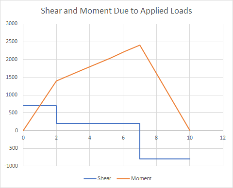
Adjustments to the end forces are found using the REAct3D function, previously described here.  The procedure is:

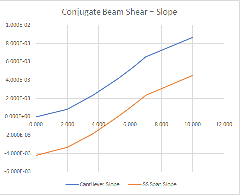
  1. For each principal axis, find the reaction force and moment at End 1, and the deflection and slope at End2 of the beam, due to the applied loading, treating the beam as a cantilever fixed at End1, with any specified spring releases.
  2. Find the deflection and rotation at End2 due to unit applied force and moment, including the effect of spring releases.
  3. Calculate the end loads at End 2 required to return the beam to zero deflection and rotation.
  4. Combine the loads from Steps 1 and 3.

Note that in the current version the spring stiffness is required to be greater than zero.  Any end release with zero or negative stiffness, or left blank, is taken as a rigid connection.

The latest version of the spreadsheet, including full open-source code, can be downloaded from: 3DFrame.zip.

See 3DFrame with spring releases for more information, including links to installation instructions for the compiled solvers.


Posted in Beam Bending, Excel, Finite Element Analysis, Frame Analysis, Newton, Strand7, UDFs, VBA | Tagged , , , , , | Leave a comment

On the probability of frog croaks.

A recent logical puzzle from TED discussed the probability of one of two frogs being female, if we know that at least one of them is male:

This puzzle is discussed (arriving at different conclusions) here:

and puzzles of this type even have their own Wikipedia article:

Boy or Girl paradox

People discussing this problem tend to fall into one of two camps, and are convinced that the other camp is completely wrong, but the correct answer depends not just on what information is given in a particular version of the puzzle, but also on the factors that control what information is given.

To summarise the TED puzzle, a man has to decide if he is more likely to find a female frog in a group of two, one of which croaks like a male, or a single  frog that is not croaking.  The problem is that we do not know if female frogs croak, the frequency of croaking, or if being in a group of two affects the rate of croaking, but all these things affect the answer.

The explanation in the TED video appears to assume that only male frogs croak, and that when in a group of two, only one will croak, although this is not stated explicitly.  Based on this they calculate a probability of 2/3 for one of the two frogs being female, but only 1/2 for the single frog being female.

The discussion at the second video on the other hand states that:

frogriddle1

… so which (if either) is right?

One way to find out is to carefully tabulate all the possibilities, and calculate the probabilities of each, which is the approach used in the video links, arriving at different answers.

A simpler approach is to set up a computer simulation of the problem, and see what numbers come out, which is what:
Frog Croaks.xlsb
does.

The spreadsheet setup is shown below:
frogriddle2

The spreadsheet is set up to model any situation where it is required to find a female, either from a group of 2 (assumed to be on the left), or a single specimen on the right.  Obviously it could also be applied to any other situation with a binary choice and a 50/50 frequency.  For each sample the spreadsheet generates 1000 random numbers between 0 and 1, and assumes a male for numbers below 0.5, or female for above.  The following options are provided:

  • Cell C1 is the “cut-off score”.  The spreadsheet generates a second random number.  If this is below the cut-off score the sex of the sample  is treated as being known, otherwise it remains unknown.  In the frog context this is equivalent to the frog croaking or not croaking.
  • Cell E1 controls whether the cut-off score is applied to males only (only males croak), or both male and female (both croak, but with different croaks).
  • The spreadsheet includes a macro to do multiple repeats of the analysis, for  a range of different cut-off scores.  Enter the number of repeats in cell P2, press Alt-F8, and select the “Repeats” macro.
  • Results for a single run are displayed in cells K2 and L2, showing the probability of a female in the group of 2, on the left, and from the single sample on the right.
  • The same results from the repeat analyses are in columns S and T, and in the graph below.

The screen shot above shows results if only male frogs croak, with a cut off score (equivalent to the probability of any individual male frog being heard to croak) in the range 0.1 to 0.8.  It can be seen that the probability of a female increases from just over 50% to over 83%, but it is the same for the group of two (with a single croaking frog) and the single un-croaking frog.

If we assume that females croak at the same rate as males (with a different distinctive croak) then the probability of a female frog reduces to 50% for both the pair of frogs and the single frog, as shown below.  The rate of croaking now makes no difference to the probability of a female, which makes sense because it is now assumed that females croak at the same rate as males:frogriddle3

So are there any circumstances where the conclusion reached in the original video (that the pair of frogs with at least one male is more likely to have a female) is correct?  This would require that only males croaked, they only croaked when in a pair, and there was a 50% chance of a male frog in a pair being heard to croak.  Under those conditions the probability of a female in the pair of frogs would be 2/3 (as stated in the TED video), and the probability of the single frog being female would be 1/2.

None of these details are stated or implied in the puzzle statement however, so the correct answer is that the man should go for the single frog on the right, since it is easier to catch and lick one frog than two.

Posted in Excel, Maths, Newton, VBA | Tagged , , | Leave a comment

Chris Hadfield reviews 2016

Canadian Astronaut, Commander Chris Hadfield, reminds us of all the great many positives that happened in 2016. :

It’s easy to forget that this year saw a great many positives

Posted in Bach, Newton | Tagged | Leave a comment