Non-linear Frame Analysis

Another example using Fortran code published in Programming the Finite Element Method (5th ed. John Wiley & Sons, I.M. Smith, D.V. Griffiths and L. Margetts (2014)), this post provides a spreadsheet based frame analysis program including non-linear bending behaviour and 2D or 3D analysis, linking to Fortran solver functions, via Python and xlwings.  Note that at present the spreadsheet has only rudimentary functionality for post-processing and plotting of results, and only provides input for loads at nodes, so for linear analysis the spreadsheets Frame4 and 3DFrame provide better functionality.

The new spreadsheet and related files, including full open source code, may be downloaded from:

NonLin-Frame.zip

To run the spreadsheet, in addition to Excel, the requirements are:

  • Python, including Numpy, Scipy and Ctypes
  • Xlwings
  • The provided compiled Fortran files, Main.dll and Geom.dll may be installed anywhere on the system path, or in the same directory as the spreadsheet and Python files.

The simplest way to install the required Python modules is to install Anaconda Python, which includes xlwings.  The program has been tested with Python 2.7.  It should work with Python 3, but if not, please let me know.

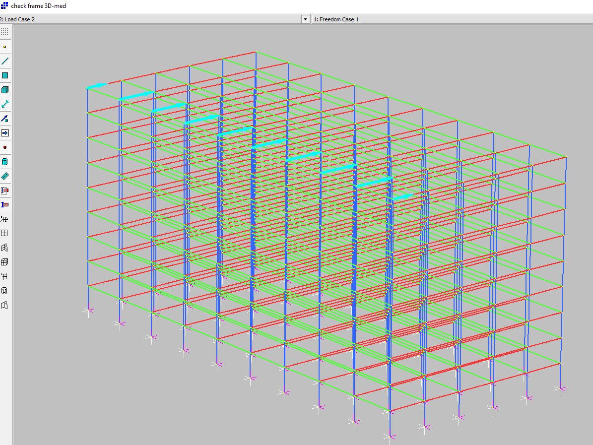
The program is based on Program P45 from Edition 5 of Programming the Finite element Method.  The beam elements are treated as elastic – perfectly plastic, and specified nodal loads may be factored in any number of load increments.  The download file includes data for the 3D frame analysis shown below:

NL-Frame1-7

Data is input on the spreadsheet, with any number of material types, nodes and beam elements (up to the 1 million+ rows provided by Excel):

NL-Frame1-1

Forces and moments are applied at nodes only in the current version.  Specified loads are factored by any number of load increments:

NL-Frame1-2

Input for 2D analyses is in a similar format, with data restricted to the available freedoms (X and Y directions, and moments about the Z axis):

NL-Frame1-3

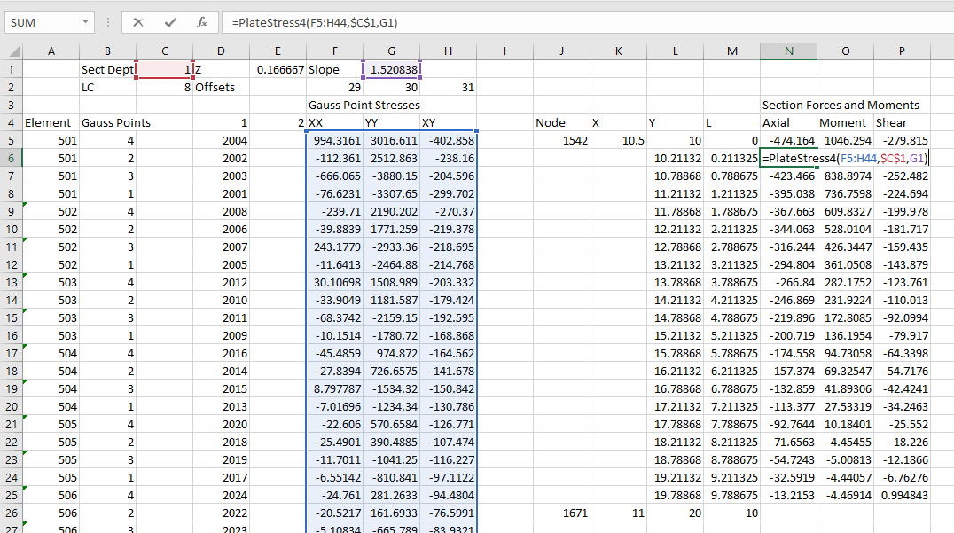
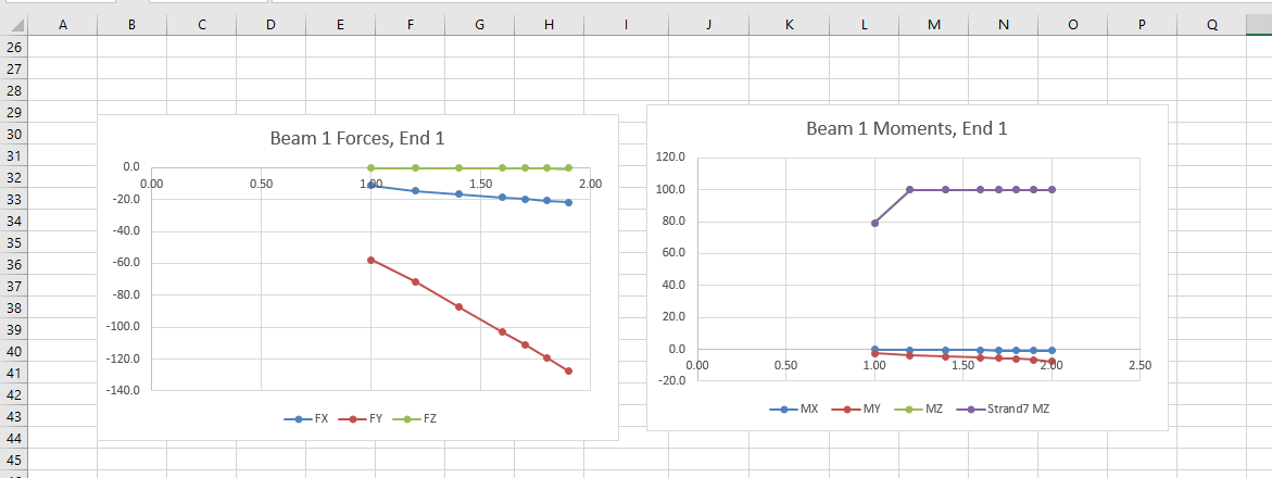
The analysis is run by clicking a button on the “Results” sheet.  Full lists of node deflections and beam end actions are copied to the “Deflect” and “StressRes” sheets respectively.  At present the “Results” sheet only provides a brief summary of each load increment, and plots of deflections for one node, and forces and moments for one beam, with up to 8 load increments.  This will be extended in later versions.

NL-Frame1-4

The example output also plots X deflection and Z-axis moment results from the finite element analysis program Strand7, using the same elastic-plastic beam properties.  It can be seen that there is good agreement between the two, although not exact due to different methods of modelling the non-linear behaviour.

NL-Frame1-5

Strand7 provides a facility to re-number nodes, to improve the efficiency of the matrix solution process.  Three different node numbering sequences have been copied to the spreadsheet, and it can be seen below (row 7) that the solution times for this medium sized frame are almost unchanged.  For a larger frame (2730 Nodes and 7065 beams) the “tree” node sequence was about four times faster than the other two options.

NL-Frame1-6

Posted in Beam Bending, Excel, Finite Element Analysis, Fortran, Frame Analysis, Link to dll, Link to Python, Newton, NumPy and SciPy, Strand7, UDFs, VBA | Tagged , , , , , , , , , , | 5 Comments

Darrell Scott & Danny Thompson

Playing at HebCelt 2013 in Stornoway.

Don’t forget the headphones:

… and a slightly older recording featuring Danny Thompson with Pentangle (who were Jacqui Mcshee, Bert Jansch, John Renbourn and Terry Cox)

Posted in Bach | Tagged , , , | Leave a comment

ConbeamU 4.10

The ConbeamU spreadsheet has been updated to Version 4.10, to fix a problem with incorrect default parameters being used if the support stiffness columns had empty cells.  The revised spreadsheet (including open-source code) can be downloaded from:

ConbeamU.zip

Applications in the spreadsheet include:

Conbeam and ConbeamU; continuous beam analysis with any number of supports and beam segments.  Supports may have specified translation or rotation stiffness or specified displacements.  ConbeamU (and other functions ending in U) are unit aware, allowing input and output in a wide variety of different units:
CobBeamU10-1

There are also similar functions for single spans (SSSpanU) and cantilevers (CantileverU).

MovLoadU does moving load analysis on a continuous beam, with vehicles with any number of axles:

CobBeamU10-2

FEAU and REAU find fixed end moments or restrained end moments for a single span with fixed ends or spring restrained ends.  The beam may have any number of segments with different section properties.

ConBeamU-REA

Any number of loads may be applied, which may be point forces or moments, of uniform or trapezoidal distributed loads:

ConBeamU-REA2

The BeamAct3D function returns beam actions and deflections along the beam, for a beam with any number of segments and specified end conditions and applied loads.

CobBeamU10-3

The React3D function returns fixed or restrained actions for a beam with any number of segments, subject to 3D loading:

CobBeamU10-4

Download the spreadsheet for more details of each function, and information on using array functions.

Posted in Beam Bending, Excel, Finite Element Analysis, Frame Analysis, Newton, Strand7, UDFs, VBA | Tagged , , , , , , , , | 24 Comments

Retaining wall analysis – FEA and hand calculations

I have used the PlateMC spreadsheet described in the previous post to compare the results of a finite element analysis of a retaining wall with a similar analysis using the commercial package Strand7, and a simple hand calculation using Coulomb soil pressure theory.

The spreadsheet may be downloaded from:

PlateMC-dll-staged.zip

The finite element model used is shown in the screen-shot below, showing the deformed shape under final load, with 100 times magnification of displacements:

PlaneStrain7-3

The main features of the analysis were:

  • The retaining wall was a 10 metre high reinforced concrete structure, with an 8 metre wide base.
  • Different soil properties were assigned to the foundations, the fill elements immediately behind the wall, the remaining elements over the wall heel, and the remaining fill.
  • The fill was placed in 2 metre high layers, with a 20 kPa compaction load applied and then removed from each layer.
  • The final load case included a 30 kPa surcharge load, over the full width of the fill top surface.
  • The spreadsheet and Strand7 analyses used the same soil properties, except that the first spreadsheet run included a dilatency angle for the fill elements.

The hand calculation used a fixed active pressure coefficient, Ka, based on the standard Coulomb equation, using the properties of the fill over the heel:

PlateMC-RW1-Coulomb

For this structure the wall back face angle to the vertical (omega), and the top fill surface angle to the horizontal (beta) were both zero.  The fill friction angle (phi) and the soil/wall interface friction (delta) are listed in the screen shots below, together with the fill elastic modulus values used in the finite element analyses.

The results shown below are all for the completed fill plus 30 kPa surcharge load.  The first analysis used the same elastic modulus value for all the fill (50 MPa), and equal friction values of 35 degrees for the structural fill and the friction layer:

PlateMC-RW1-1

The Plate MC and Strand7 results were similar over most of the wall, but the Strand7 results increased more quickly towards the base, with the moment at the base being about 8% higher.  The hand calculation was about 20% higher than the Strand7 results.

Results of setting the soil dilatency angle to zero in the PlateMC analysis are shown below:

PlateMC-RW1-2

Bending moments at the base were slightly increased, but the results are still about 6% lower than the Strand7 results.

Reducing the elastic modulus of the general fill to 20 MPa slightly increased the PlateMC bending moment, and reduced the Strand7 moment, such that the results at the base were very close:PlateMC-RW1-3

Reducing the friction angle of the friction layer (and the hand calculation delta angle) to 17.5 degrees increased both finite element analyses by about 20%, with the PlateMC results now being a little higher.  The hand calculation moment was reduced a little (about 1%), reducing it to less than the FEA results.

PlateMC-RW1-4

Reducing the elastic modulus of the friction layer to 20 MPa had only a small effect, increasing the Strand7 moment slightly and reducing it for PlateMC:

PlateMC-RW1-5

Reducing the wall friction to zero in the hand calculation increased the bending moment by about 8%, to a value just over that found in the finite element analyses with a 17.5 degree friction layer:PlateMC-RW1-5a

Reducing the friction angle of the friction layer to 10 degrees increased the maximum bending moment in the FEA results by about 20%:PlateMC-RW1-6

Removing the compaction loads from the finite element analyses had only a small effect on the results, slightly reducing maximum bending moments for both programs:PlateMC-RW1-7

In summary:

  • Results from the spreadsheet, PlateMC_staged, and Strand7 were reasonably consistent, especially with reduced friction angles for the friction layer.
  • Maximum bending moments from the hand calculation were significantly higher than the finite element results when the full friction angle was used.
  • Reducing the friction layer friction had much less effect on the hand calculation results than the FEA results.
  • Reasonably consistent results were found (in this case) when the FEA results with friction zone angle of 17.5 degrees were compared with the hand calculation results with zero interface friction.
Posted in Excel, Finite Element Analysis, Fortran, Frame Analysis, Geotechnical Engineering, Link to dll, Link to Python, Newton, NumPy and SciPy, Strand7, UDFs, VBA | Tagged , , , , , , , , , , , , , | Leave a comment

Plane Strain FEA – Non linear staged analysis

Continuing the recent series of posts featuring Fortran based FEA routines, the spreadsheet from the previous post has been revised:

  • The spreadsheet allows for a staged analysis, with additional elements placed in layers for any number of construction stages.
  • Temporary loads may be applied to the top surface of each layer, and then removed.
  • The mesh details are entered as node coordinates, and plate node numbers, rather than the automated mesh generation methods used previously.
  • The PlateStress4 user defined function (UDF) has been added, allowing beam forces and moments to be extracted from the Gauss Point stresses of plate elements.

The new file, including full open-source code, may be downloaded from:

PlateMC-dll-staged.zip

As before, the spreadsheet requires Python (including Numpy) and xlwings, all of which are included in the free Anaconda Python package.

Example input and results are shown below, featuring analysis of a 10 metre high cantilever retaining wall, with fill placed in 5 stages:

PlaneStrain7-1

Any number of materials may be defined.  Properties are:

  • E: Young’s Modulus
  • v: Poisson’s Ratio
  • c: Cohesion
  • phi: Friction angle
  • psi: Dilatency angle
  • gamma: density (force units)

All plates are 8-noded plane strain elements, with nodes defined in the clockwise direction, starting at the bottom left corner.

PlaneStrain7-2

The construction sequence is defined with the last plate number in each applied layer (column W).  Both plate and node numbers must form a continuous sequence in each layer.  Compaction loads (column Z) are applied to then removed from the top surface of the plates listed in columns X and Y.  The final layer may also have a surcharge load applied to the specified plates as the final load case.

Restrained nodes are indicated with 0 for restrained freedoms and 1 for unrestrained.

Any number of pairs of nodes may be pinned, forcing equal X and Y deflections.

PlaneStrain7-3

Typical results for the example structure are shown above.  The next post will provide more details of results of different soil properties, and also compare results with those from a commercial FEA package (Strand7), and standard retaining wall analysis procedures.

PlaneStrain7-4

Numerical summary results are shown above, including results after placing each layer, and after application and removal of the compaction load.  Total execution time was just over 5 seconds.

PlaneStrain7-5

The spreadsheet is set up to calculate the axial force, bending moment, and shear force over the height of the wall for any specified load case.

PlaneStrain7-6

Calculation of the wall actions is carried out on the ConcRes sheet.  The procedure to generate these results is:

  • List the element numbers where results are required, with 4 rows for each element.
  • Calculate the row and column numbers from the StressRes range for the required Gauss points and load case.
  • Use the Index function to return the required stress values.
  • Use the PlateStress4 function to calculate the axial force, bending moment, and shear force for each of the selected plates (see previous post)
Posted in Beam Bending, Concrete, Excel, Finite Element Analysis, Fortran, Geotechnical Engineering, Link to dll, Link to Python, Newton, NumPy and SciPy, UDFs, VBA | Tagged , , , , , , , , , , , | 1 Comment