Dynamic charts

A frequently asked question is how to get Excel charts to automatically update when new data is added outside the original selected ranges. The most frequent recommendation (such as here) is to convert the data to a table, then insert a new chart linked to the table. Adding new data immediately below the table will then automatically extend the table range, and the chart will automatically update.

This post looks at an alternative approach using range names defined with a formula, plotting data defined in a dynamic array. The process is described in detail at Engineer v Sheep, including some catches in the set-up process, and how to avoid them. This post looks at an engineering related example, including a modification to deal with data outside the dynamic array.

The requirement is to plot two graphs showing bending moments and shear forces, for multiple load cases, plotted against axial load, around a reinforced concrete arch, together with the bending and shear capacity (click image for full size view):

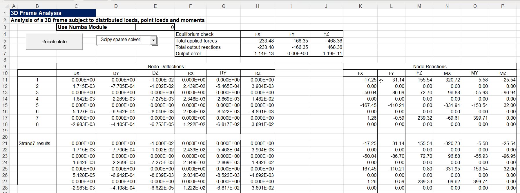
The data in the first three columns is imported from an external FEA program with VBA code. The other columns divide the moments and shear forces into three groups, depending on the sign and the reinforcement at the section. This data is returned by a user defined function, as a dynamic array.

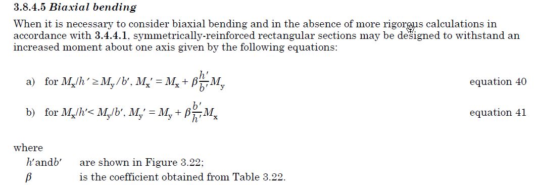
To define the ranges for plotting, each column must be given a range name defined with an index function:

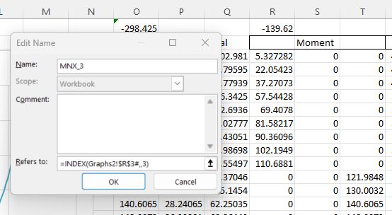
Note that the row number argument is left blank, so the function returns the whole column.

The index function can be used for all six columns returned by the UDF, but the axial loads are to the left of the UDF, and cannot be accessed using Index. For this column the Offset function must be used, with a negative row offset:

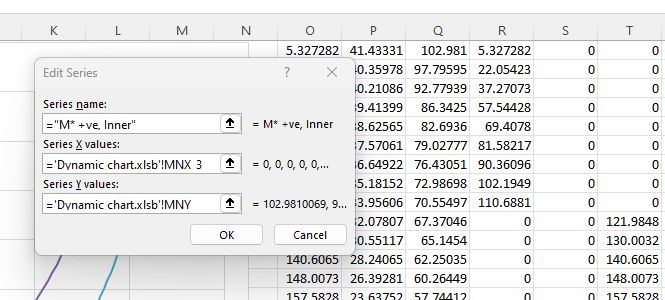
The named ranges can then be used to define the graph ranges:

Posted in Charts, Charts, Concrete, Excel, UDFs | Tagged , , , , , | Leave a comment

Simplified bi-axial bending

This post summarises my responses to a question at Eng-Tips.

The UK concrete standard in use before Eurocode 2 (BS 8110) has a simple procedure for designing columns subject to bending about both principal axes:

This allows the column to be designed to resist a factored moment about one axis.

Eurocode 2 has a different approach:

AS 3600 follows the same approach as Eurocode 2, but with slightly different exponent factors:

The Eurocode/AS 3600 procedure requires the section capacity to be checked about both axes, but it’s actually quite easy to derive an equation for the minimum resistance moment for the axis with the larger moment, similar to the BS8110 one:

For applied moment Me and moment resistance Mr, if Me/Mr is equal about the two axes then Equation 5.39 reduces to:

2(Me/Mr)^a <= 1.0

So for minimum Mr: (Me/Mr)^a = 0.5

Me/Mr = 0.5^(1/a)

Mr = Me/(0.5^(1/a))

In the graph below I have plotted 1/(0.5^(1/a)) with 1 + Beta from BS8110, the equivalent factor from the Australian code (AS 3600), and the factor derived from the biaxial analysis of a square section with equal moments about both axes, for a range of axial loads:

The factor is applied to the design bending moment, so a higher factor is more conservative.

The graph below shows the ULS bending capacity about one axis for a square section with equal applied moment about both axes. The section details were:

  • Dimensions: 600 x 600
  • Reinforcement; 4 N20 bars each face, yield strength = 500 MPa
  • Concrete: 40 MPa, cover 40 mm

Increasing the steel diameter to 40 mm has a significant effect on the results, with the simplified methods being much less conservative under high axial loads, and very unconservative under very high axial loads:

Posted in Excel | Leave a comment

3DFrame-py

My 3DFrame spreadsheet has now been converted to Python code and can be downloaded from:

3DFrame-py.zip

The frame analysis uses the Scipy linear algebra functions called from pyLinalgfuncs3, which must be available on the Python path:

pyLinAlgfuncs3.zip

The 3DFrame-py download file includes:

  • 3DFrame-py.xlsb: The basic spreadsheet, including data for a small example frame
  • 3DFrame-py Strand7 check.xlsb: Results for the small frame compared with Strand7 results.
  • 3DFrame-py-vvbig.xlsb: Spreadsheet with input and results for a much larger frame
  • Load3DFrame.py: Python code to load the 3DFrame-py code at startup of the associated spreadsheet
  • py_3DFrame0_1.py: The 3DFrame-py code, using the Numba just-in-time compiler.
  • py_3DFrame0_1-nojit.py: The same code but without any calls to Numba jit compilation.

In addition to the download files, the following modules are used:
Required:

  • pyxll
  • Numpy and Scipy
  • ctypes

Optional:

The spreadsheet has VBA code to automatically load the Python frame analysis code when the file is opened:

Public Sub Workbook_Open()
Dim iErr As Long

Application.EnableEvents = True
iErr = Run("Load3DFrame")
End Sub

The Load3DFrame module should either be added to the list of files opened at startup, in the pyxll.cfg file, or the code below should be added to an existing startup file:

import pyxll
from pyxll import xl_menu, xl_macro, xl_app, xlcAlert
import importlib as imp

@xl_macro
@xl_menu("Frame Analysis", menu="Load")
def Load3DFrame():
    xl = xl_app()
    usejit = xl.Range("Usejit").Value
    try:
        if usejit == 0:
            imp.import_module('py_3DFrame0_1-nojit')
        else:
            imp.import_module('py_3DFrame0_1')
        pyxll.rebind()
        xlcAlert('Frame Analysis module import completed')
    except:
        xlcAlert('Module not imported')
    return 0

The Python code is a work in progress, and the functionality of the spreadsheet is largely the same as the VBA version. The major differences are that the links to compiled solver routines have been replaced with links to the Scipy and pyPardiso solvers, and there is now an option to use code calling the Numba just-in-time compiler:

For large problems using the Numba module greatly reduces the time to complete an analysis, but the first time the solver is used the compiled code takes about 20 seconds to generate, so for small frames (or if the Numba module is not available), it is better to leave it disabled.

The spreadsheet has been saved with data for a small frame, and the results are compared with the Strand7 FEA results, showing near exact agreement:

The spreadsheet is able to handle much larger frames, and the download file has an example with nearly 10,000 nodes and over 27,000 beam members:

Note that for models of this size the Numba code should be enabled, and the solver should be set to one of the 2 iterative options, or to Scipy sparse, if the pyPardiso module is installed. The banded solver is very slow for models of this size, and may have memory overrun problems.

Background information on the methods used to generate and solve the frame model can be found by selecting “Frame Analysis” from the Categories drop down list at the top-right of the blog Home tab.

Posted in Arrays, Excel, Finite Element Analysis, Frame Analysis, Link to Python, Newton, NumPy and SciPy, PyXLL, Strand7, VBA | Tagged , , , , , , , | 3 Comments

More new old recordings

There have been quite a few old Pentangle and Bert Jansch recordings posted on YouTube in recent months.

BBC The Genius of Bert Jansch Folk Blues and Beyond, from 2014. Interviews and archive footage weave together performances from a concert at the Royal Festival Hall celebrating the songs and artistry of the folk-blues troubadour Bert Jansch.

Pentangle – ‘Newsnight’ 26/06/08:Robin Denselow investigates to third coming of the five and has coffee by the Thames with publishing personality Ian Anderson.

A Guardian article about the same concert:

Pentangle’s 2008 Royal Festival Hall reunion brought them back to the venue of the live half of their Sweet Child double album (1968). By many accounts, that performance was not without its rough edges. But the musicianship on display during tonight’s two-set engagement is awe-inspiring, virtuosic and – still – somewhat perverse: an endless knot of strings, disparate influences and textures.

And a Bert Jansch concert at the same venue in the early days: Bert Jansch – Royal Festival Hall 30/6/71

Posted in Bach | Tagged , , , | Leave a comment

Calculating and plotting rotations

This post was prompted by a recent post at Eng-Tips.

The original problem seemed simple enough:

Im trying to wirte a formula where I imput vessel heading and datum bore heading and it tells me FWD, STBD, AFT or PORT

Now FWD and AFT are I can manage. If the difference between two headings is 45 or less then its FWD. if its greater than 135 its AFT

Between 45 or 135 is PORT or STBD depending on which way vessel turns. If vessel turns clockwise on compass then bore heading on PORT and and if anticlockwise its STBD

Anyone know how to write such a thing on excel?

For consistency the terminology used in the rest of this post will be:

  • Angles are measured clockwise from North, so will always be between 0 and 360 degrees.
  • The angle from the boat to the datum bore is referred to as the Reference Bearing.
  • The ship’s direction of travel is referred to as the Heading
  • The angle required is the angle from the Heading to the Reference Bearing, which will be divided into FWD, STBD, AFT, PORT, and back to FWD, with transitions at 45, 135, 225, and 315 degrees.

The problem is that if the angle is calculated as Ref. Bearing – Heading, it may lie between -360 degrees and 360 degrees, which makes any single formula using nested if statements very long. The simplest solution is to use a VLookup formula with a table, as in the screenshot below:

The table can be shortened by using the formula =MOD(Ref-Head, 360), which returns an angle between 0 and 360. The shortened lookup table is in my opinion the simplest solution, and the easiest to check, but two working alternatives were given in the discussion, which used a single cell formula:

  • The formula in cell A16 uses =INDEX() with a list of the four direction names, and a formula using MOD() that returns a value between 1 and 4.
  • The formula in cell A11 uses the sum of the Sin and Cos of Ref-Head, together with nested Ifs and ANDs.

A simpler solution using the ABS function was suggested, but this does not work when the Ref-Head angle is negative.

Finally Eng-Tips regular MintJulep provided some VBA code to plot the Reference Bearing and Heading instantly whenever one of the angles was changed:

Both spreadsheets shown above, including full open-source VBA code can be downloaded from:

Bearings.ZIP

Posted in Coordinate Geometry, Drawing, Excel, Maths, Newton, VBA | Tagged , , , , , , | Leave a comment