This is probably widely known, but I only found out this week.
I find You-tube informative videos frustrating because you have to sit through 10-20 minutes of video to get maybe 1-2 minutes worth of information. If only you could display a transcript of the spoken words!
Well it turns out you can:
Click on the three dots below the bottom right corner of the video, and select “show transcript”
… and the transcript is displayed to the right. You can then click on the three vertical dots to the top-right of the transcript and select toggle time-stamp.
You can then read the transcript on-line, or select and copy to a word-processor or text editor.
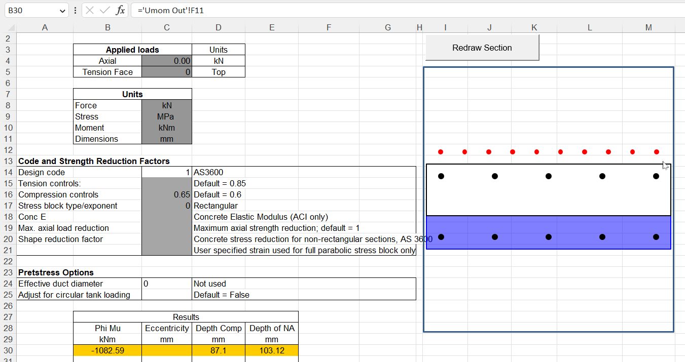
The main new feature is the option to design for prestress loads applied to circular tanks. Due to axi-symmetric effects, when circumferential prestress is applied to a circular tank structure this generates a uniform axial stress across the cross section, in spite of the eccentric position of the prestress cables. This is handled by applying a virtual reaction moment, equal and opposite to the moment due to the eccentricity of the prestress. Use of this feature is illustrated in the screenshots below (click any image for full-size view):
If the “Adjust for circular tank loading” is set to “False”, or left blank, the section capacity is calculated in the usual way, allowing for the eccentricity of the prestress force:
If the option is set to True, the virtual moment is applied to the section, reducing the section capacity:
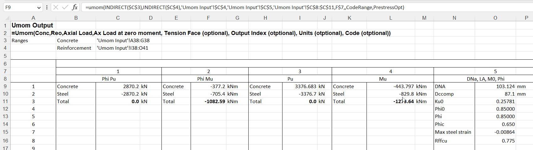
The correction for the circular tank effect is shown in the function output:
Following the first post in this series, this post compares friction losses in prestressing cables as defined in the Australian Concrete Structures Code (AS 3600), compared with a cable modelled with contact elements in Strand7. The example used is based on the same three span beam used in the previous post (taken from the book Concrete Structures by Warner, Rangan, Hall and Faulkes), but the cable profile has been modified over the internal supports to provide a more realistic profile:
In the Strand7 analyses the prestress was applied by applying a strain preload to additional elements at each end of the cable, representing the stressing jacks. The strain was adjusted to generate a force of 1500 kN at each end of the cable.
Friction in AS 3600 is defined by:
As in the previous post, the friction curvature coefficient was taken as 0.2, and the wobble factor as 0.016.
In Strand7 the frictional behaviour of the contact elements is controlled by two factors:
The friction coefficient
The “sticking friction stiffness”: For Zero Gap and Normal Gap elements with non-zero coefficients of friction, the Sticking Friction Stiffness provides the lateral elastic connection between nodes until the point where the element slips in the lateral (frictional) direction; while the frictional force is below the current frictional capacity the lateral elastic stiffness is added.
There is little guidance on how the Strand7 sticking friction stiffness should be determined, and as far as I know, no guidance on how it relates to the AS 3600 “wobble factor”. A range of values have therefore been used, and the results of the Strand7 FEA and the AS 3600 formula compared.
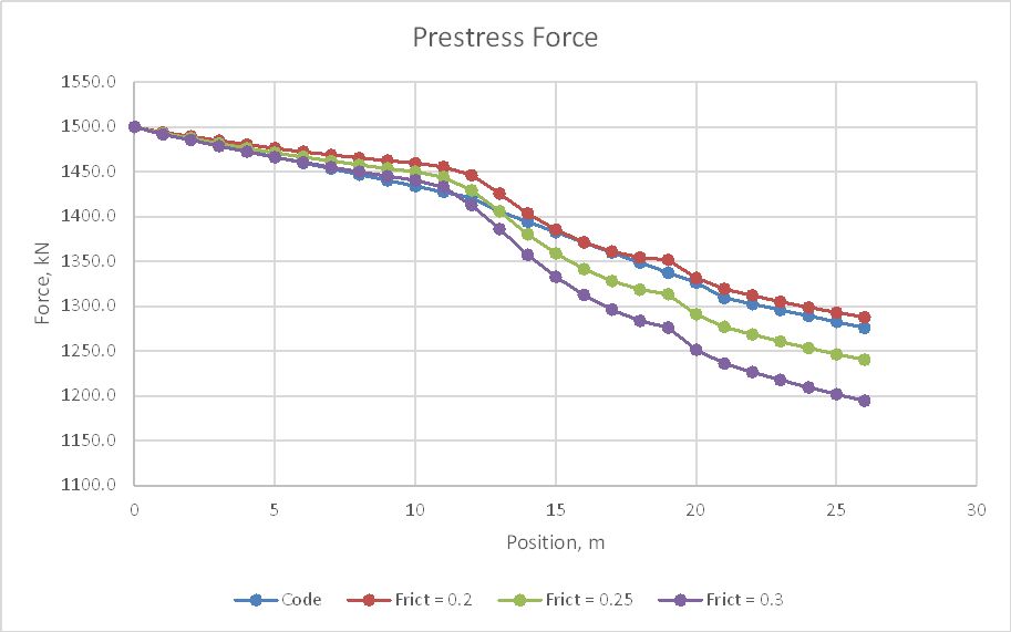
The friction factor was initially varied between 0.2 and 0.3, with a constant sticking friction stiffness of 10,000 kN/m. The resulting tendon forces from one end to mid-length are shown below:
Over the first ten metres, where the cable profile had a low curvature, the AS 3600 formula gave slightly higher friction losses than the FEA with 0.3 friction factor, but over the remainder of the length all FEA results had higher friction losses and the friction factor of 0.2 was the best overall fit.
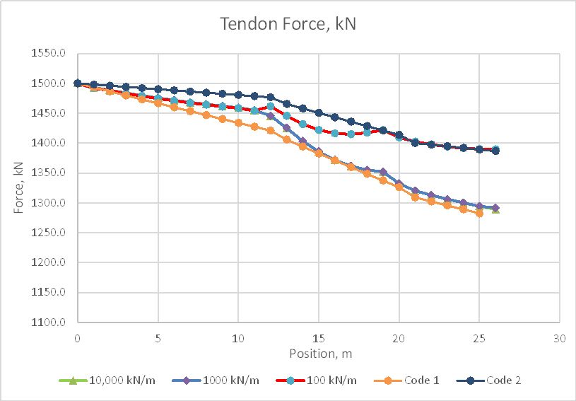
The analysis was then run with a friction factor of 0.2, and sticking friction stiffness values of 10,000 kN/m, 1000 kN/m, and 100 kN/m. The AS 3600 formula was checked with a wobble factor of 0.016 (Code 1) and 0.0 (Code 2):
All three of the FEA results are very close, up to 11.0 metres, where the 100 kN/m diverges to meet the Code 2 line. The other two lines remain very close over the full length, and are a good match with the Code 1 line from 14 metres onwards.
The above analyses were continued by reducing the strain in the jack elements by 5%, resulting in approximately 8 mm shortening of the elements, representing the loss of jack force due to lock off of the strands. In the graph below line 4a is the 10,000 kN/m line without the reduction in prestress:
Now all three runs with different sticking friction values have significantly different results over the full length. The effect of these differences on the bending moments in the beam will be examined in the next post in this series.
Ana Vidović (born 8 November 1980) is a classical guitarist originally from Croatia. A child prodigy, she has won a number of prizes and international competitions all over the world.
Here she is at St. Mark’s Church, San Francisco:
Concert starts at 2:00
PROGRAM:
Flute Partita in A minor, BWV 1013 by Johann Sebastian Bach (Transcribed by Valter Despalj) -Allemande (3:06) -Corrente (8:40)
Violin Sonata No. 1, BWV 1001 by Johann Sebastian Bach (arr. by Manuel Barrueco) -Adagio (12:44) -Fuga (16:38) -Siciliana (21:19) -Presto (24:25)
Un Dia de Noviembre (27:36) by Leo Brouwer
Gran Sonata Eroica, Op. 150 (32:17) by Mauro Giuliani
Sonata in E major, K. 380, L. 23 (41:39) Sonata in D minor K.1, L. 366 (46:28) by Domenico Scarlatti
The beam analysis functions in the ConbeamU spreadsheet allow for the use of any SI units, or any non-SI units found in the long list included with the spreadsheet. I usually use all SI units, but in this case I was wanting to use kip and foot units with the SSSpanU function, and found that the function did not work with the units as entered, and did not provide any indication of the problem. To improve that, I have added to the list of non-SI units (as described below), and modified the code so that it gives a more helpful message when input units are not recognised. The updated spreadsheet can be downloaded from:
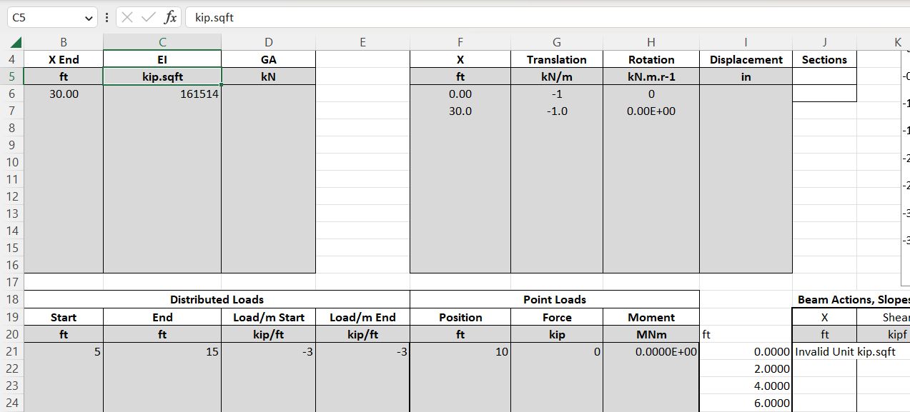
The Eng-Tips discussion linked above concerned ways of finding the maximum deflection of a beam under non-symmetrical loading. This can be easily done using the SSpanU function together with the Excel Solver. A similar procedure can also be used with the ConBeam function. Input for an example beam is shown below (click image for full size view):
Input and output units have been set to kip and feet units, with output deflections in inches.
Unused inputs (support stiffness and point moment loads) have been left as SI units. These would normally be set to the same units as the other inputs, although mixed units will be converted and calculate correctly without a problem.
Output was originally set to display at 2 foot intervals, as listed in column I
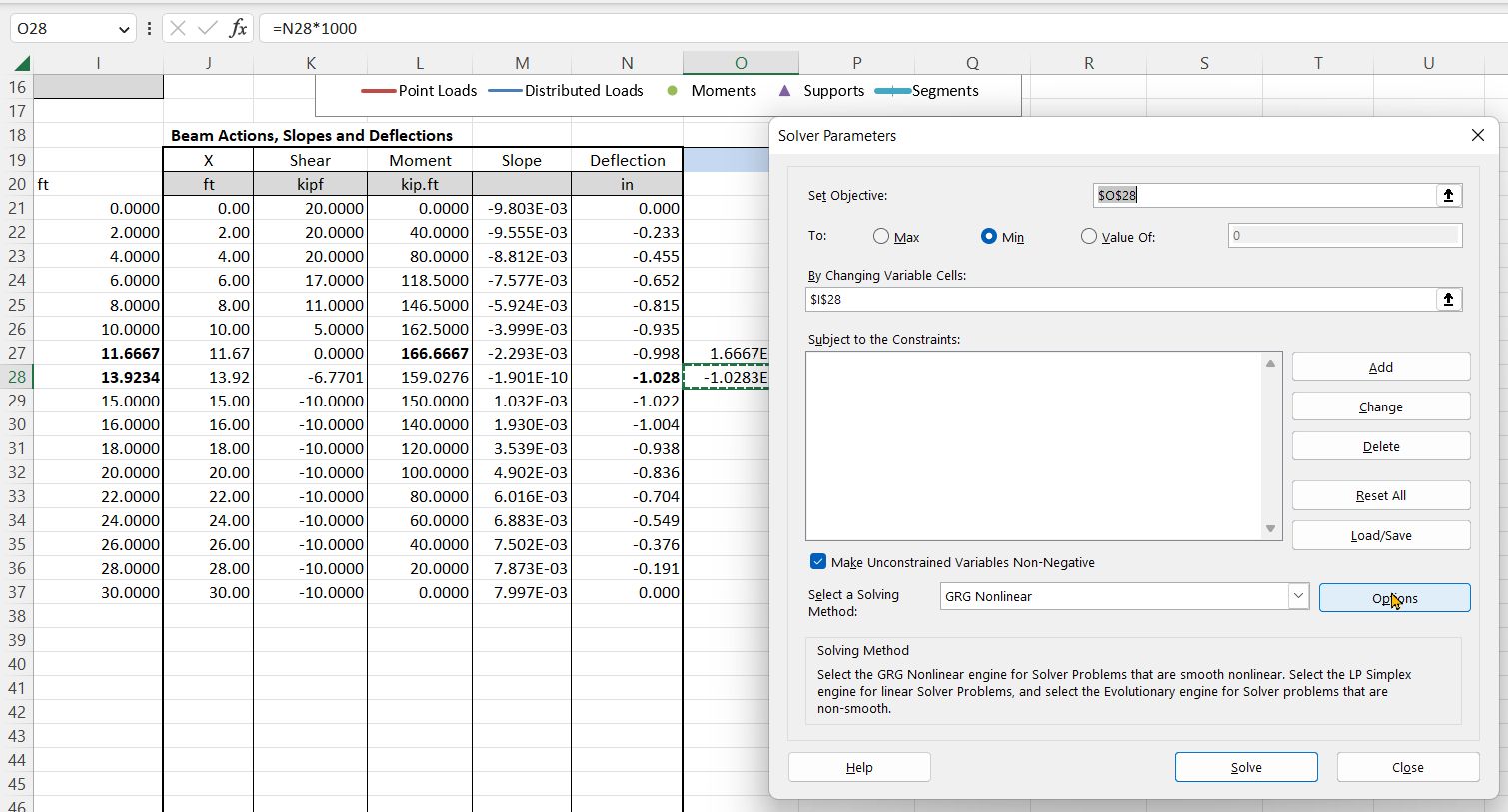
The screenshot blow shows the Solver input to find the point with maximum deflection. In general, with non-symmetric loading, this will not be at mid-span or at the point of maximum bending moment.
By inspection, the maximum deflection was seen to be between 13 and 14 ft from the left support. To use the Solver the deflection output for 14 ft has been multiplied by 1000 in cell O28. This is used as the Solver “objective value”. The Solver is set to minimise this value by changing the output location in cell I28. The Solver adjusts the value to 13.9234, with a deflection of -1.028 inches.
There are two reasons for using the factored value in O28, rather than the function output in N28:
The SSSpanU function is entered as a dynamic array in cell J21. Excel displays the whole output array, but the Solver function does not recognise the cells other than J21 as containing a formula. You therefore need to enter another formula outside the array range, referring to the cell you want to maximise or minimise.
For results that have a small numerical value such as deflections the Solver default tolerance may result in an inaccurate result.
The location and value of the maximum bending moment is found in a similar way, except the formula in cell O27 does not factor the moment value, and the Solver is set to maximise this value.
The latest version of the units functions now returns a more helpful message if it does not recognise one of the supplied units, as shown below:
The non-SI units list has now been modified to recognise the following abbreviations:
kip or kipf is recognised as 1000 lbf
Bending moments may be entered with a space (kip ft) or a point (kip.ft) and using kip or kipf
Flexural stiffness (EI) may be entered as kipf.ft2, kip.ft2 or kip ft2
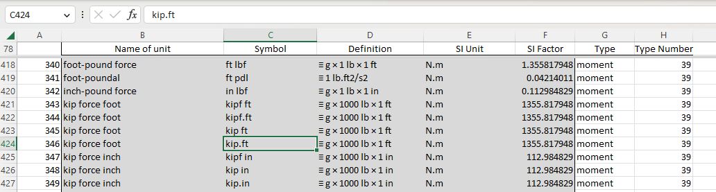
Non-SI units are listed on the Ext Unit List sheet. Adding new abbreviations to this list is easy. The example below shows kip.ft added to the list:
Find the unit type you want to add to (e.g. “moment”).
Insert a blank row below one of the existing units in that row.
Copy the row above down into the new row.
Enter the new unit abbreviation under Symbol (Column C).
Check that columns E to H are copied correctly, and that the SI Factor is correct.