Secondary moments in prestressed beams with FEA

Secondary (or hyperstatic) bending moments occur in prestressed beams that are continuous over internal supports, or have other redundant support conditions. Any eccentric prestress force will cause a beam to deflect, and if these deflections are restrained at internal supports, this will generate additional bending moments, known as secondary or hyperstatic moments. This post looks at alternative ways of modelling these effects in an FEA program (Strand7), and compares the results with simpler beam analysis procedures. The example used is taken from the book Concrete Structures by Warner, Rangan, Hall and Faulkes.

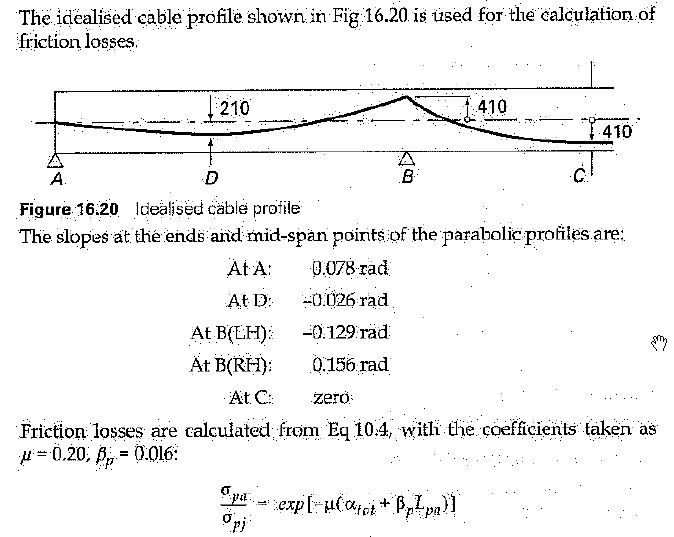
The beam consists of 3 spans, with lengths of 16 m, 21 m, and 16 m, and with post-tensioned reinforcement with parabolic profiles as shown above. The cable is assumed to be stressed at both ends, with an applied force of 1494 kN. The variation of force along the cable, calculated to AS 3600 friction losses, is shown in the graphs below.

The following methods were used to find the bending moments along the beam due to the prestress force, including secondary moments:

  • 1: Apply prestress loads directly to beam; apply friction losses to AS 3600
    a: Apply vertical loads to nodes on prestress cable profile, connected to beam with rigid link.
    b: As a) + horizontal loads.
    c: Apply point moments to beam at mid-segment locations.
    d: As c) but apply moments at segment ends.
  • 2: Include prestress cable in the model, apply preload to the cable.
    a: Connect cable to beam with rigid links, apply prestress as uniform average load, cable modelled as string group of truss elements.
    b: As a) except include friction losses to AS 3600
    c: As b) except no string group. Apply prestress as 3 uniform loads based on average load for each span.
    d: As c) except cable modelled with beam elements.
    e: As d) except links modelled with beam elements
    f: As c: except prestress applied with friction losses to AS 3600
  • 3: Include prestress cable, apply loads to the end of the cable. Cable modelled as beam elements, connected with friction contact elements.
    a:) End loads applied as pre-strain applied to “jack elements”.
    b:) End loads applied as point loads applied to the cable ends and equal and opposite loads to the beam ends.

The analysis results shown below were generated with the Strand7 FEA program. Note that other programs may return significantly different results, especially for models including “string groups” or friction elements. The graphs below show the axial force along the prestress cable, compared with the calculated forces applied to the Type 1 beams. Results are shown for the left hand half of the beams, which are symmetrical about the mid-length.

The force distribution for all the Type 1 beams was calculated according to AS 3600. The step in the diagram is due to the deviation in the cable profile at the internal supports. A revised example with a more realistic profile will be examined in a later post, but for now the simplified profile has been maintained for consistency with the book calculation.

For beams 2a and 2b the prestressing cable was modelled as a string group, which behaves as a cable passing over frictionless pulleys, so any applied forces are equally distributed over the length of the cable. For beam 2a the average force from the AS 3600 distribution was applied over the full length. For beam 2b each beam segment in the model was assigned a different force, but these have been averaged over the string group, resulting in a slightly higher average force than my calculation.

For beam 2c the cable was not modelled as a string group, but as a series of truss elements, connected to the beam with rigid links. The cable in each span was allocated the average force for that span. The interaction of the prestressed cable with the beam concrete resulted in the line shown above.

Beams 2d and 2e were similar to 2c, except they were modelled with beam elements, rather than truss elements, and 2e was connected to the main beam with beam elements rather than rigid links. All 3 generated very similar loads along the cable.

Beam 2f was the same as 2c, except that a different prestress force was allocated to each segment. This has resulted in a profile following the trend of the AS 3600 line quite closely, but with a reduced force. In a later post the applied prestress force will be adjusted to allow for the distribution of the prestress force into the concrete.

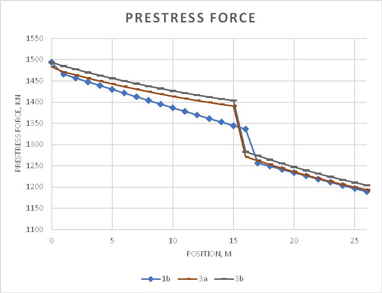
Beams 3a and 3b were both modelled with beam elements connected to the main beam with friction elements and rigid links. The prestress force was applied to the ends of the cables, through a pre-strain applied to beam elements representing the stressing jacks for Beam 3a, and with direct axial forces applied to the ends of the cable for Beam 3b, with equal and opposite forces applied to the ends of the main beam. In both cases there were significantly reduced prestress losses in the end spans, compared with AS 3600, but the loss at the support was greater, and forces for the middle span were well matched. It should be possible to get a closer match to the AS 3600 forces by adjusting the friction element parameters. This will be examined in a later post.

The results for all beams are summarised below, showing the calculated prestress force at mid outer and internal spans, and bending moments due to the prestress at mid-spans and at the internal piers. The beams were also analysed with no internal supports, and the difference between these two values is the secondary moment.

Of the four models where prestress actions were applied directly to the main beam, 1b is the most accurate since this included the effects of horizontal loads. Comparing the other models with 1b:

  • The models using a string group for the prestress cable (2a and 2b) had exactly equal prestress force over the beam length, even when the applied force was varied along the length. This results in significantly different behaviour, the main difference in this case being higher bending moments in the central span.
  • The three models without string groups, but where the prestress was applied as the average load over each span (2c, 2d, 2e) gave better results, but the prestress distribution was still significantly different from model 1b, which may result in significant errors in some cases.
  • For model 2f the prestress was applied as a different load for each segment. The resulting load followed the trend of loads calculated with AS 3600 friction losses, but was significantly lower over the full length, resulting in significantly lower bending moments at each section, compared with 1b. In future analyses the prestress load will be adjusted for this case, so that loads are equal to the required values after transfer.
  • Models 3a and 3b had friction contact elements connecting to the main beam, with prestress loads applied as a strain in an element representing the stressing jack, or as applied end forces. In this case the end loads were adjusted so that they matched the required force at the beam ends, but the parameters used for the contact elements resulted in lower friction losses over the end spans.

In the next post in the series models 2f, 3a and 3b will be investigated in more detail to provide a better fit of the cable forces to that found using AS 3600 friction losses. The cable profile will also be modified over the internal supports to follow a realistic profile for a continuous cable.

Posted in Beam Bending, Concrete, Excel, Finite Element Analysis, Frame Analysis, Newton, Strand7 | Tagged , , , , , , | 1 Comment

Which was Douglas Adams’ single best line of writing?

is a question from Quora, from which my favourite of the many responses was:

Although I am a huge fan of The Hitchhiker’s Guide to the Galaxy in all its incarnations and have been quoting from it nearly all my life, I think Douglas’s single best line of writing actually comes from The Salmon of Doubt (a collection of previously published and unpublished material that was published one year after his untimely death):

This is rather as if you imagine a puddle waking up one morning and thinking, ‘This is an interesting world I find myself in — an interesting hole I find myself in — fits me rather neatly, doesn’t it? In fact it fits me staggeringly well, must have been made to have me in it!’ This is such a powerful idea that as the sun rises in the sky and the air heats up and as, gradually, the puddle gets smaller and smaller, frantically hanging on to the notion that everything’s going to be alright, because this world was meant to have him in it, was built to have him in it; so the moment he disappears catches him rather by surprise. I think this may be something we need to be on the watch out for.

For many more see: https://www.quora.com/Which-was-Douglas-Adams-single-best-line-of-writing

Posted in Newton | Tagged , | Leave a comment

Downloads from the 60’s

Two new download sites with some of my favourite music from the 1960’s:

Bert at the BBC from bandcamp:

https://bertjansch.bandcamp.com/album/bert-at-the-bbc

… and for something completely different, assorted recordings from Tom Lehrer:

Posted in Bach | Tagged , , , | Leave a comment

py_UMom spreadsheet and OptShearCap3600 function

I have now transferred the Ultimate Limit State design functions from the VBA RC Design Functions spreadsheet to Python format. The new spreadsheet and Python code can be downloaded from:

py_UMom.zip

The code also includes the OptShearCap3600 function, described in the previous post.

The python code requires pyxll to connect to Excel. If this is installed, and “RC_UMom” is added to the list of modules to load at start-up in the pyxll.cfg file, the new functions should be available from any spreadsheet.

The included functions are:

py_UMom: ULS design of rectangular sections with two layers of reinforcement under combined bending, axial load, shear and torsion, to Australian and international codes. (Provision for prestressing will be added in the near future):

py_UmomPF: As above, but for Eurocode and British codes using a partial factor approach:

MaxAx: Maximum axial load for short or slender columns:

Devlength: Reinforcement development length to Australian, Eurocode, or British codes:

ShearCap3600: Shear capacity to current AS 3600 and 5100.5:

OptShearCap3600: Optimise shear capacity for given moment/shear ratio by adjusting the compression strut angle:

Extracts of the OptShearCap3600 function code are shown below. The scipy.optimize.brentq function is used to adjust the applied loads to be equal to the design section capacity:

# create list of arguments for the py_Umom function, called by the Scipy brentq function
    args = [InCells, Puin, 13, 1, Muin, [] , ShearReo, Code, VTuin] 
    
    # Use scipy.optimize.brentq to adjust the input shear force to be equal to the design capacity
    try:
        res  = sopt.brentq(call_Umom, mincap, maxcap, args = args, maxiter = 100)  
    except:
        outA[0,0] = 1
        return outA

# The call_Umom function adjusts the input loads in proportion to the shear force 
#  passed by brentq, then calls py_Umom and returns the difference between the 
#  applied shear and shear capacity

def call_Umom(Vstar, args):
    args[8][0,0] = Vstar
    args[4][0] = Vstar * MoV
    if ToV != 0: args[8][0,1] = Vstar * ToV
    if PoV != 0: args[1][0] = Vstar * PoV
    res = py_Umom(*args )
    return res[1]

Similar procedures are used to adjust the applied moment when this is critical, or the compression strut angle in the intermediate range, so that both shear and moment capacities are equal to the applied actions.

Posted in Excel | 1 Comment

More on combined shear and bending design to AS 3600

Further to the last post on this subject I have been looking at procedures to speed up design for shear to AS 3600 when the “refined” analysis procedure is used. The issues that need to be addressed are:

  • The design shear capacity reduces with increasing tensile strain at the mid-depth of the section, and the tensile strain increases with increasing applied moment and shear force. To find an accurate upper limit to the shear capacity it is therefore necessary to carry out an iterative analysis to match the applied shear force, and associated bending moment, with the shear capacity of the section. This is particularly important for the assessment of existing structures, where it is a requirement to find the actual maximum capacity of the structure, rather than designing for predefined maximum loads.
  • The maximum shear capacity may be controlled by the shear failure or by the combined effect of bending, shear and torsion on the longitudinal force on the tensile reinforcement.
  • As discussed previously, where the section capacity is controlled by the longitudinal tension force the design capacity can be increased by increasing the angle of the shear compression strut. This also requires an iterative process.

I have now written a Python function to carry out the iterations using the Scipy brentq function with the procedure outlined below:

  1. From the input data calculate the ratios: moment/shear (M/V) and torsion/shear (T/V)
  2. Adjust the shear force and associated actions so that the applied shear force equals the design shear capacity.
  3. If the design bending capacity, reduced for the longitudinal force due to shear and torsion, is greater than the applied moment then return the results, else:
  4. Set the shear compression strut angle to the maximum value allowed by the code (50 degrees) and adjust the shear force and associated actions so that the applied moment is equal to the reduced design bending capacity.
  5. If the design shear capacity is now greater than the applied shear force then return the results, else:
  6. Adjust the shear compression strut angle so the ratios Applied Shear/Design Shear Capacity and Applied Moment/Design Moment Capacity are equal.
  7. Adjust the shear force and associated actions so that the applied shear force equals the design shear capacity.
  8. Repeat 6 and 7 until the ratio of applied actions/design capacity equals 1 for both shear and bending.

Typical function output is shown in the screenshot below:

In this example the section has been analysed for a constant shear force with an increasing M/V ratio. The function output (Columns K to O) is:

  • Design shear capacity, and the associated bending moment for the input M/V ratio.
  • The “excess capacity” for shear and bending. Note that this has three zones where the capacity is initially controlled by shear only, then both shear and moment are at full capacity, then the adjusted bending capacity controls.
  • The compression strut angle (Theta). The strain values in Column P are calculated with a simple on-sheet formula.

These results are plotted below with typical shear and bending loads, taken from a heavy road vehicle travelling over an 8 metre simply supported span, with the loads plotted at 0.4 and 1.0 metres from the support. The capacity is also plotted with no adjustment of the compression strut angle, showing a significantly reduced capacity.

Plotting the section capacity as a moment-shear interaction diagram allows the loads from all sections with identical reinforcement to be plotted on the same section, and load cases where the applied loads exceed the section capacity are immediately visible.

This is a work in progress, but a spreadsheet with all necessary Python files will be available for download shortly.

Posted in Beam Bending, Concrete, Excel, Link to Python, Newton, NumPy and SciPy, PyXLL, UDFs | Tagged , , , , , , , , | 4 Comments