Latex Maths Text in Excel

There have been many posts here looking at alternative ways of working with functions entered as text on a spreadsheet, and working with units, most recently here.

One drawback with this approach is that text in an Excel cell must be ASCII or Unicode, which has limited capabilities for presenting maths text in a readable form. Excel does allow elaborate maths equations to be generated and displayed, but as far as I know there is no way to interact with these equations from VBA, so they can neither be generated by code, or evaluated by code.

Python on the other hand has libraries that will convert plain text equations to Latex (and other formats), and display Latex code. I have now written a Python function “plot_math” using a combination of Sympy, Pint, and Matplotlib to:

  • Read any maths function from the spreadsheet
  • Convert the text to Latex format
  • Return a graphic image of the function
  • Optionally evaluate the function using a table of values for each parameter
  • Optionally adjust for the units of the input and output values.

The new code can be downloaded from:

EvalU.zip

The spreadsheet requires the following software:

  • Python
  • pyxll
  • Numpy
  • Scipy
  • Pint (which includes sympy and mpmath)
  • Matplotlib

The download file includes two Python files:

  • startup_min.py
  • py_Units4Excel.py

Startup_min.py includes the plot_math function, and should be added to the list of files to open at start-up in pyxll.cfg.

Note that this is a work in progress. If you have any problems with installation or running the programs, please let me know.

Some examples of the new function in action are shown below:

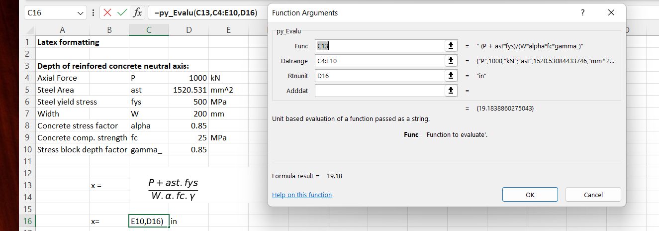
The text to be displayed (and optionally evaluated) should be entered as plain text at any chosen location. In the example below the plot_math function is then entered in the cell immediately above (C12).

When the plot_math function is entered the image will display immediately below:

The image can then be dragged to the desired location; in this case so that the original text and the function return value (0) are hidden. In this example the numerical value of the function for selected input values is displayed using the py_Evalu function.

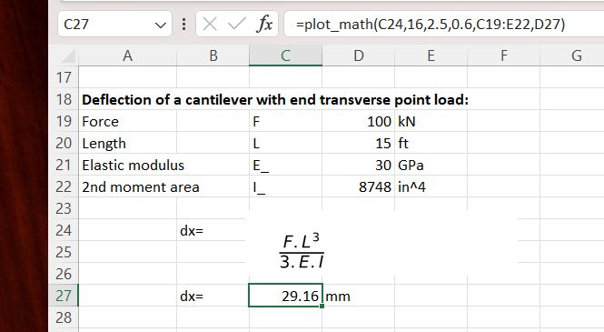
Alternatively the plot_math function will return the value of the function if suitable input data is selected:

In this case a three column data range has been selected, and also an output unit, so the calculation will be unit aware:

As before, the image is displayed immediately below the plot_math input cell, but can be dragged to any desired location:

Some other features to note:

  • If the data range has only two columns (variable name and value) the calculation will have no units.
  • If the output unit is omitted, and the data range has three columns including units, the output value will be in base SI units.
  • Names of Greek letters (e.g. alpha) will generate the Greek character
  • In some case Greek letter names will be the name of a standard maths function (e.g. Gamma), in which case the text should be followed by an underscore (gamma_)
  • Some English letters also represent standard maths values (e.g. e and i). If an upper-case E or I is required, these should be entered followed by an underscore, and will then be displayed in upper-case, without the underscore.
  • The exponentiation symbol may be entered in either Excel (^) or Python (**) format. In either case the exponent will display as a superscript, and the calculation will be correct
Posted in Excel, Link to Python, Maths, Newton, NumPy and SciPy, PyXLL, UDFs | Tagged , , , , , , , , , , | Leave a comment

Go Your Way

We haven’t had any Bach for a bit, so here is:

An excellent cover of Anne Briggs’ song, Go Your Way:

And Anne Briggs herself singing the song, accompanied by Bert Jansch:

Go Your Way Anne Briggs

And another cover (posted here 12 years ago yesterday):

Posted in Bach, Excel | Tagged , , | Leave a comment

RC Design Functions 9.03; compression strut angle adjustment

The RC Design Functions spreadsheet has now been updated to Version 9.03, and is available for free download from:

RC Design Functions9.zip

The new version includes a number of corrections to the calculation of beam shear and torsion capacity to AS 3600 and AS 5100.5:

  • Shear capacity under negative bending moments has been corrected.
  • The sign of reported shear capacity is now the same as the input shear force (previously any input with negative moment returned a negative shear capacity).
  • The contribution of any negative torsion to longitudinal tension forces, to AS 3600, was taken as zero. This is actually in accordance with equation 8.2.7(3) of the code (since Amendment 2), but clearly the absolute value of the torsion should be used.

In addition, the new version allows the minimum angle of the concrete compression strut to be specified, between 29 and 50 degrees. The specified angle is used to calculate a minimum value for the mid-depth strain, which is also used in the calculation of the kv factor. Increase in the mid-depth strain value is allowed under Cl. 8.2.4.2 in both AS 3600 and AS 5100.5.

Use of the compression strut angle adjustment is shown in the screen-shots below:

A beam has design loads of 400 kNm bending moment, and 275 kN shear force. With 10 mm shear reinforcement the shear capacity is just adequate, but taking account of the longitudinal forces due to shear the bending capacity is reduced to 371 kNm:

Increasing the shear reinforcement to 14 mm diameter increases the shear capacity, but using the code calculated compression strut angle to AS 3600 the reduced bending capacity is unchanged. (Note that AS 5100.5, and earlier versions of AS 3600, have a substantial increase in the bending capacity when the shear reinforcement is increased. This is discussed further below):

Entering a compression strut angle of 49.6 degrees (with the “Use simplified” option set to “False”) reduces the shear capacity back down to the required value (275 kN), but the moment capacity is now increased to 416 kNm. Note that any further increase in the shear reinforcement would have negligible effect (to AS 3600) because the compression strut angle is already very close to the maximum value of 50 degrees:

The effect of increasing the shear reinforcement on the adjusted bending capacity with different codes and approaches is shown in the graph below:

The lines are:

  • 1) AS 3600, Amendment 2 or 3, default compression strut angle.
  • 2) AS 3600 with compression strut adjusted to maintain constant shear capacity.
  • 3) AS 5100.5, default compression strut angle.
  • 4) AS 5100.5 with adjusted compression strut angle.
  • 5) As 3), but shear reinforcement force limited in accordance with the Canadian Bridge Code.

So what is going on here?

In AS 5100.5 (and AS 3600 up to Amendment 1) the longitudinal force due to shear is defined as:

Vus is proportional to the area of shear steel, and is not limited, so increasing the shear steel area allows the value of DeltaFtd to be reduced to zero, even though in reality the actual force in the steel cannot be greater than the applied shear force (V*) minus the concrete shear force. The large increase in bending capacity with increased shear steel shown by line 3) is therefore not realistic.

Increasing the compression strut angle (Thetav) with the AS5100.5 equation reduces cot(Thetav), which reduces Vus, but also reduces DeltaFtd. The resulting calculated bending capacity is still unrealistic for large areas of shear reinforcement.

In AS 3600 Amendment 2 the equation for longitudinal force due to shear was revised to:

If the shear capacity of the section is exactly equal to V* then this equation is equivalent to the AS5100.5 version, but increasing the area of the shear reinforcement has no effect on Vuc, so there is no reduction in DeltaFtd, and the bending capacity remains constant, as seen in line 1.

In this case however increasing Thetav, which reduces cot(Thetav) reduces both Vuc and the resulting value of DeltaFtd. Increasing the shear reinforcement area therefore allows Thetav to be increased (so that the shear capacity remains equal to the design shear force), which reduces DeltaFtd, with the nett result that the bending capacity is very close to the values found from the AS 5100.5 equation, until Thetav reaches the upper limit of 50 degrees, after which the bending capacity remains constant (line 2).

Finally the Canadian Code requires the value of Phi.Vus to be limited to V*. In this case this restriction is more conservative than the approach taken in AS 3600. Bending capacities are similar to the other results for small shear reinforcement areas, but the maximum bending capacity is significantly lower than that found with AS 3600 with adjustment of the compression block angle.

In summary:

  • The AS 3600 equation with default compression block angle is conservative, but shows no benefit from increased shear reinforcement area.
  • Applying adjustments to the compression block angle, in accordance with the code, the AS 3600 equation gives results very close to those from AS 5100.5, up to a reasonable limit (i.e. maximum angle of 50 degrees, equivalent to a maximum mid-depth strain of 0.003).
  • If the shear reinforcement area is increased well above the area required for the design shear force the AS 5100.5 equation gives bending capacity results that are highly unconservative.
  • If design is required to follow the current AS 5100.5 (Amendment 1), it is recommended that the Canadian code limit (Phi.Vus < V*) be applied.
Posted in Beam Bending, Concrete, Excel, Newton, UDFs, VBA | Tagged , , , , , , , , | 2 Comments

Linking to Python help from Excel

The py_Numpy spreadsheet presented in the previous post has been updated:

  • A large number of Numpy functions added.
  • Return function help documentation to the spreadsheet for a selected function.
  • View Numpy on-line documentation from the function Wizard.

The new version can be downloaded from:

py_Numpy.zip

As before, the pyxll add-in is required for the connection from Excel to Python.

All the available functions are listed on the first sheet. Enter the index number for a function in cell F4, and the help for that function will be displayed:

The on-line help for all the listed Numpy functions can also be accessed quickly and easily through the Function Wizard.

Select a function and click on the “Insert Function” icon (immediately to the left of the Edit bar):

Then click “Help on this function” in the bottom left corner:

The Numpy on-line help for the selected function is displayed.

Note that this is a work in progress. Connecting to the on-line help requires a different html path to be generated for each function, and the path names are not always consistent. If you find any Numpy functions where the help is not displayed, please let me know.

Posted in Excel, Link to Python, Newton, NumPy and SciPy, PyXLL, UDFs | Tagged , , , , , , | Leave a comment

Calling Numpy polynomial functions from Excel

The Numpy polynomial related function discussed in recent posts can now be downloaded from:

py_Numpy.zip

The download file includes Python code and a sample spreadsheet. Required installed software is Python, Numba and pyxll to call the code from Excel. Some of the functions in the default file require the just-in-time compiler, Numba. For those without Numba installed the file pyNumpy-noJIT.py can be used.

Note that the Quadratic, Cubic and Quartic functions (which are not included in Numpy) are based on C code from the following sources:

The screenshots below show examples of the spreadsheet functions: (click on any image for full-size view).

The py_PolyRoots function calls the general purpose Numpy function, that will work for any degree polynomial. The alternative functions have very much better performance for degrees up to quartic.

Py_PolyFromRoots finds polynomial factors from its roots. Py_PolyVal returns the function value for any value of x, allowing array input.

Py_PolyFit fits a polynomial to input data:

Other Numpy polynomial functions are shown below:

The py_flip functions reverses a Numpy array along a specified axis:

Finally functions are provided to form a Numpy array of complex numbers from an Excel list of pairs of floats:

Posted in Curve fitting, Excel, Link to Python, Maths, NumPy and SciPy, PyXLL, UDFs | Tagged , , , , | 1 Comment