Solving non-linear equations with two or more unknowns – 5

This will be the last of the series on solving non-linear equations (for now).  Up until now all the examples have had two unknown values, and two target values.  This can be extended by making three changes to the code:

  • Set up an nxn matrix of the function slopes with respect to each of the unknown values (the function Jacobian)
  • Calculate the first estimate of the target values, using an estimated value for each of the unknowns.
  • Form and solve a series of simultaneous equations to find a better estimate of the unknowns.

In Excel VBA the solution to the equations can be found using the Worksheetfunction.MInverse and MMult functions, as shown in the code below:

LoopNum = LoopNum + 1
        ' Evaluate function at guessed values and small increments.
                                            
        For i = 1 To NumVar
            Var2A(i, 1) = Var1A(i, 1) * VarFact
            VarDiffA(i, 1) = Var1A(i, 1) * (VarFact - 1)
        Next i
        Res1 = Application.Run(Func, Var1A, X)
        For j = 1 To NumVar
            ResDiff(j, 1) = Target(j, 1) - Res1(j, 1)
        Next j
        Temp = Var1A(1, 1)
        Var1A(1, 1) = Var2A(1, 1)
        For i = 1 To NumVar
            Res2 = Application.Run(Func, Var1A, X)
            
            For j = 1 To NumVar
                SlopeA(j, i) = (Res2(j, 1) - Res1(j, 1)) / VarDiffA(i, 1)
            Next j
            Var1A(i, 1) = Temp
            If i < NumVar Then
                Temp = Var1A(i + 1, 1)
                Var1A(i + 1, 1) = Var2A(i + 1, 1)
            End If
        Next i
        
        ' Solve SlopeA
        InvA = WorksheetFunction.MInverse(SlopeA)
        ResA = WorksheetFunction.MMult(InvA, ResDiff)
        
        ErrSum = 0
        For i = 1 To NumVar
            ErrA(i, 1) = (Target(i, 1) - Res1(i, 1))
            ErrSum = ErrSum + Abs(ErrA(i, 1))
            Var1A(i, 1) = Var1A(i, 1) + ResA(i, 1)
        Next i

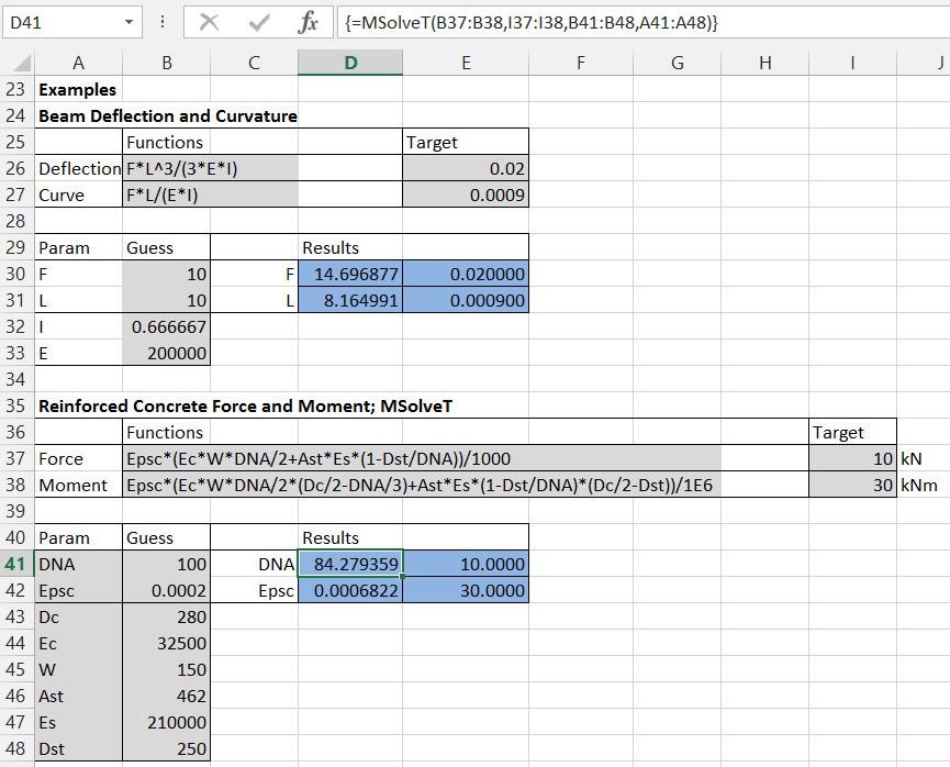
The User Defined Function (UDF) MSolve has been modified as shown above, and the earlier version renamed MSolve2.  A spreadsheet including examples of both functions, and full open source code, can be downloaded from:

Eval2.zip

Input and output from both functions is shown in the screenshot below:

Solve2var-15

MSolve2 works as before, in the example returning the depth of neutral axis and compression face strain in a reinforced concrete section, for any given axial load and bending moment.

The MSolve example adds one more unknown (the diameter of the tension reinforcement), and another target, the tension reinforcement stress.

The Python Scipy package also contains a number of routines for solving problems of this type.  In order to access these from Excel we need:

  • A python routine for the function to be solved.
  • An interface allowing this routine and the Scipy functions to be accessed from Excel.

I have updated the Eval-PyIntegration spreadsheet to perform this task, and this can be downloaded from:

Eval-PyInt.zip

The spreadsheet uses ExcelPython for communication with Python, and the download file includes all necessary files (other than Excel, Python and Scipy).

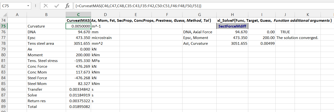
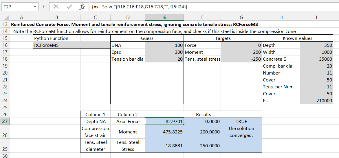
The example below shows the xl_SolveF function used to find the depth of neutral axis, compression face strain, and tension bar diameter required for a specified axial force, bending moment and tension steel stress.  In this example the Python function being solved (RCForceMS) is the simplified version, ignoring concrete in tension.

Solve2var-16

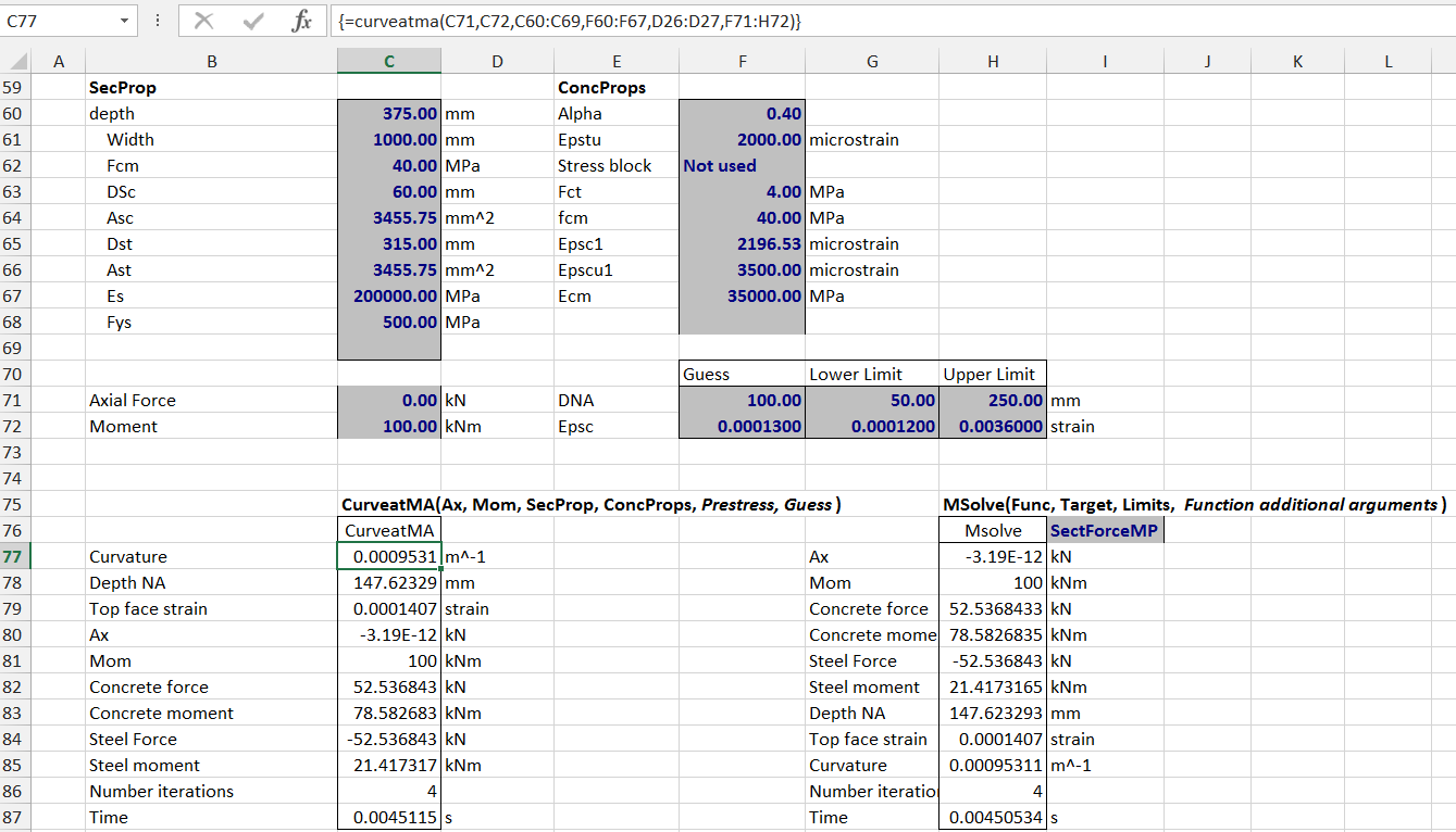
The download also includes Python versions of the functions CurveatMA and CurveatMAS, with input as shown below.  The functions make use of the SciPy optimize.root function, which has many optional arguments, detailed in the SciPy manual.  In the spreadsheet the only options included are for the solver type, and tolerance for termination.

Solve2var-17

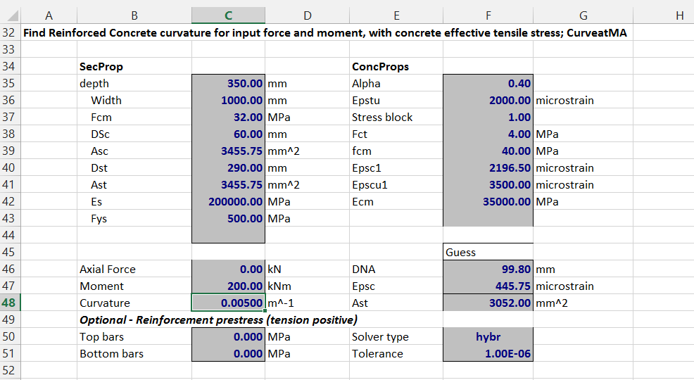
The screenshot below shows the results of CurveatMA for an axial load of zero and bending moment of zero.  The returned values of depth of neutral axis (DNA) and compression face strain (Epsc) have been checked using the function SectForceMV, which finds that the axial force and bending moment are as expected.

The xl_SolveF function can also be called directly, using a function that returns the difference of the function values from the target values, in this case SectForceMDiff.

Solve2var-18

Finally, CurveatMAS adjusts the neutral axis depth, compression face strain, and tension steel area such that the axial force, bending moment and section curvature match the target values.  Once again, xl_SolveF may be used with SectForceMdiff to return the same 3 values.

Note that the steel force and tensile strain found by these functions are average values, including tension stiffening effects.  The results are intended for use in deflection calculations, and should not be used in strength or stress limit calculations.

Solve2var-19a


Posted in Beam Bending, Concrete, Excel, Link to Python, Maths, Newton, NumPy and SciPy, UDFs, VBA | Tagged , , , , , , , , , , , , | 3 Comments

Solving non-linear equations with two or more unknowns – 4

As promised in the previous post, the spreadsheet including the new functions to calculate reinforced (or prestressed) concrete moment-curvature with a revised concrete tension stress-block is now available for download from:

RC design functions7.zip

The spreadsheet includes full open source VBA code.

Use of the new functions is illustrated in the screen-shots below:

The function MomCurveTS returns a table of bending moment and curvature results (and associated output).  The required input is the section properties data, the axial load, and the Alpha (f’t/ft) and Epstu values defining the effective concrete behaviour in tension (see here for more details).  The remaining properties may be entered by the user, or enter -1 to use the Eurocode 2 default values, based on the value of fck entered under SectProps.  Reinforcement prestress, and the number and range of output steps may also be specified.

Solve2var-10

The function returns the section curvature at zero moment (which will be non-zero if eccentric prestress is applied), just below and just above the cracking moment, and then at equally spaced steps up to the compressive strain specified in StepA.

For each moment the function also returns:

  • The depth of the Neutral Axis
  • The “top ” (i.e. compression) face strain
  • The axial load (constant, equal to the input value)
  • The effective Elastic Modulus
  • The curvature given by the Eurocode 2 empirical formula
  • The cracked curvature with no tension stiffening.

Solve2var-11

Typical results are shown in the graph below:

Solve2var-12

The MomCurveTS function uses the function CurveMA to find the section curvature at just above the cracking moment.  It then increases the compressive face strain in equal increments and returns the associated moment and curvature.  CurveMA uses the Function MSolve to find the compressive face strain and depth of Neutral Axis for any combination of axial load and bending moment (within the section capacity), and these functions may be called directly from the spreadsheet as shown below:

Solve2var-13

MSolve calls the function SectForceMP to find the section axial force and bending moment for any given Neutral Axis depth and compression face strain.  An equivalent function, SectForceMV, may be called directly from the spreadsheet as shown below, together with two further functions: EC2ForceM which calculates the force and moment in the concrete, and Stressatx, which calculates the compressive stress in the concrete at distance X from the Neutral Axis, according to Eurocode 2 Figure 3.2:

Solve2var-14a

Posted in Beam Bending, Concrete, Excel, Maths, Newton, UDFs, VBA | Tagged , , , , , , , , | 1 Comment

Solving non-linear equations with two or more unknowns – 3

For the next stage of the non-linear solver saga I am looking at the same problem as in the previous post (finding the curvature or a reinforced concrete section under specified bending moment and axial load), but with more realistic materials properties.

For concrete in compression I will use the curve from Eurocode 2, recommended for structural analysis:

Solve2var-7

For concrete in tension I will use a modified version of the curve used in a previous post:
TStiffICE

The paper this curve was taken from suggested using the stepped linear form (labelled b above) for both cracked and uncracked sections, but some testing suggests that better results are obtained using linear properties until cracking (at a stress of ft), then the tri-linear line (with a plateau at f’t) after cracking.  At this stage a simple bi-linear approach was used for the steel stress-strain; i.e. a constant E up to the yield point, then constant stress with increasing strain.

The following VBA functions are used in the calculation:

  • Stressatx and xStressatx call EC2Stress and return the stress and stress times x, at distance x from the Neutral Axis, for any given x, strain at the compression face, and concrete properties.
  • The total force and moment about the section centroid are found by SectForceMV, which calls EC2ForceM for the concrete force and moment, and SForceM for the actions in the steel.  EC2ForceM calls GaussIntF to integrate the stresses returned by Stressatx and xStressatx.
  • CurveatMA  returns the section curvature for any specified axial load, moment and concrete properties, using MSolve to find the required depth of neutral axis and compression face strain, calling SectForceMV.
  • MSolve is also used by TStiffNL, which returns the bending moment and curvature immediately before and after cracking, then at uniform strain increments up to any specified maximum compressive strain. Msolve is used in finding the compression face strain and neutral axis depth immediately after cracking.  Thereafter the top face strain is incremented in equal steps, and the depth of the neutral axis is found using the function QuadBrentPA.

Typical output from TSiffNL is shown in the screen-shot below, followed by a graph comparing results with curvature calculated with the Eurocode 2 formula:
Solve2var-8

Solve2var-9

The RC Design Functions spreadsheet will be re-issued in the next few days, including open-source code for all the functions listed above.

Posted in Beam Bending, Excel, Maths, Newton, UDFs, VBA | Tagged , , , , , , , | 1 Comment

Solving non-linear equations with two or more unknowns – 2

The previous post presented a simple but slow procedure for solving non-linear equations with two unknowns.  In this post I will describe a much faster method, that also has the advantage that it can simply be extended to work with any number of unknowns.

Three new functions have been added to the Eval2 spreadsheet, which can be downloaded (including full open source code) from:

Eval2.zip

For help with using array functions and user defined functions see: Using Array Functions and UDFs.

Looking again at the example from the previous post:

Solve2var-1
The graph can be seen as a plan view of two 3D surfaces plotting the variation of Moment and Axial Force with Depth of Neutral Axis and Top Face Strain.  The blue line is the contour on the Moment surface where Moment = 30 kNm, and the red line is the contour on the Axial Force surface where Axial Force = 10 kN.  Where these two lines intersect is the point we are looking for.

If the curved surfaces at any point are approximated by the tangent plane at that point, then the contour for any desired value becomes a straight line, and it is easy to find the intersection of these two lines for the two chosen values.  In this example the solution requires solving a simultaneous equation with two variables, but the same approach is easily extended to any number of variables, using standard matrix algebra techniques.

The procedure for this solution method is:

  • Write a function that will return the value of the two input functions to be solved for any given value of X and Y (where in the example X = top face strain and Y = depth of neutral axis)
  • Using starting guessed values of X and Y calculate the value of the two functions at three locations: (X,Y),  (X+δX, Y), and (X, Y+δY)
  • Using these three values find the slope of each surface in the direction of the X and Y axes.
  • Using these slopes, set up two equations for the contour lines at the desired values.
  • Solve the two simultaneous equations to find a revised estimate of X and Y.
  • Repeat until the calculated X and Y values are sufficiently close to the target values.

VBA code for a User Defined Function (UDF) to carry out this procedure is shown below:

Function MSolveT(Func As Variant, Target As Variant, Guess As Variant, Params As Variant, _
        Optional Defaults As Variant, Optional CommaDec As Boolean = False)
'Solve Function for 2 unknowns

Dim Err As Double, LoopNum As Long
Dim Var1 As Double, Var2 As Double, Var1_2 As Double, Var2_2 As Double, Res1 As Variant
Dim Res2 As Variant, Res3 As Variant
Dim MaxLoops As Long, ResTol As Double, VarFact As Double
Dim SlopeA(1 To 2, 1 To 2) As Variant, Var1diff As Double, Var2diff As Double
Dim ResDiff(1 To 2, 1 To 1) As Double, ResA(1 To 2, 1 To 1) As Double, Fact As Double, ResOut(1 To 2, 1 To 2) As Variant

    If IsMissing(Defaults) Then
        MaxLoops = 20
        ResTol = 0.0001
        VarFact = 1.000001
    Else
        MaxLoops = Defaults(1, 1)
        ResTol = Defaults(2, 1)
        VarFact = Defaults(3, 1)
    End If
                                        
    If TypeName(Target) = "Range" Then Target = Target.Value2
    If TypeName(Guess) = "Range" Then Guess = Guess.Value2

    
    Var1 = Guess(1, 1)
    Var2 = Guess(2, 1)
    
    LoopNum = 0
    Do
        LoopNum = LoopNum + 1
        ' Evaluate both functions at the guessed estimates and small increments in the X and Y directions.
                                            
        Var1_2 = Var1 * VarFact
        Var2_2 = Var2 * VarFact
        
        Guess(1, 1) = Var1
        Guess(2, 1) = Var2
        Res1 = MEval(Func, Params, Guess, , CommaDec)
        Guess(1, 1) = Var1_2
        Res2 = MEval(Func, Params, Guess, , CommaDec)
        Guess(1, 1) = Var1
        Guess(2, 1) = Var2_2
        Res3 = MEval(Func, Params, Guess, , CommaDec)
                                                        
        Var1diff = Var1 * (VarFact - 1)
        Var2diff = Var2 * (VarFact - 1)
                                                
        ' Create new slope array
        SlopeA(1, 1) = (Res2(1, 1) - Res1(1, 1)) / Var1diff
        SlopeA(1, 2) = (Res3(1, 1) - Res1(1, 1)) / Var2diff
        SlopeA(2, 1) = (Res2(2, 1) - Res1(2, 1)) / Var1diff
        SlopeA(2, 2) = (Res3(2, 1) - Res1(2, 1)) / Var2diff
        
        ' Solve for new estimate of X and Y values
        Fact = SlopeA(1, 1) / SlopeA(2, 1)
        SlopeA(2, 2) = SlopeA(2, 2) * Fact - SlopeA(1, 2)
        ResDiff(1, 1) = Target(1, 1) - Res1(1, 1)
        ResDiff(2, 1) = (Target(2, 1) - Res1(2, 1)) * Fact - ResDiff(1, 1)
                                                
        ResA(2, 1) = ResDiff(2, 1) / SlopeA(2, 2)
        ResA(1, 1) = (ResDiff(1, 1) - SlopeA(1, 2) * ResA(2, 1)) / SlopeA(1, 1)
                                                
        Var1 = ResA(1, 1) + Var1
        Var2 = ResA(2, 1) + Var2
        Err = Abs(Target(1, 1) - Res1(1, 1))
    Loop While LoopNum <= MaxLoops And Err > ResTol

    ' Recalculate function values with final X and Y values

    If Err < ResTol Then
        Guess(1, 1) = Var1
        Guess(2, 1) = Var2
        Res1 = MEval(Func, Params, Guess)
        
        ResOut(1, 1) = Var1
        ResOut(2, 1) = Var2
        ResOut(1, 2) = Res1(1, 1)
        ResOut(2, 2) = Res1(2, 1)
    Else
        ResOut(1, 1) = "Did not converge"
    End If
 
    MSolveT = ResOut
End Function

With the MSolveT UDF the two functions to be solved are entered as text on the spreadsheet.  These are then passed to MEval as an array of two text function, which are evaluated, and the results returned as a 2×1 array.  Note that the new MEval function can also be used as a UDF, and will work with any number of input functions.

Examples of the MSolveT UDF are shown in the screenshot below:
Solve2var-5

Where the functions to be evaluated are too complex to enter as a single line of text on the spreadsheet, the MSolveF UDF may be used.  In this case the functions are evaluated by the VBA function named on the spreadsheet, which must return a variant array with (at least) 2 rows and 1 column.

In the example below the VBA function used, RCForceM, allows for the calculation of two layers of reinforcement, and also checks if the compression reinforcement is actually in the compression zone.

Solve2var-6
Note that this function is provided for simple example purposes only. The Estress function in the Reinforced design Functions spreadsheet provides a closed form solution to the same problem, and also makes several checks that are not included in these simple examples; for instance that the neutral axis is within the depth of the section.

In the next post in this series the SolveF UDF will be used with a more complete function for evaluating the force and moment on a reinforced concrete section, including allowance for non-linear stress-strain curves for the steel and concrete, and use of a tensile stress curve for the concrete, to model tension stiffening.

Posted in Beam Bending, Concrete, Excel, Maths, Newton, UDFs, VBA | Tagged , , , , , , | 5 Comments

Solving non-linear equations with two or more unknowns – 1

Newton’s Method is a well known iterative solution for non-linear equations with one unknown.  That is, if some value Y depends on a variable X, then we can use Newton’s Method to find X for any given value of Y.  A VBA routine performing a refinement of Newton’s Method (Brent’s Method), can be found at The Inverse Quadratic Method 3 – Brent’s Method, and a recent application using this function is at Faster Biaxial Bending.

When there are two or more unknowns things get more complicated.  An example is finding the strains and stresses in a reinforced concrete section for a given bending moment and axial load, with non-linear materials properties, including effective tensile stresses in the concrete.  When the materials are treated as linear-elastic, and tension in the concrete is ignored, there are closed form solutions to this problem (see Using RC Design Functions – 1), but where the concrete and/or steel behaviour may be non-linear, and tension in the concrete is included, an iterative solution is required, adjusting  the neutral axis position, and maximum concrete compressive strain until the required bending moment and axial load are found.

The simplest procedure is to alternately adjust one variable, keeping the other constant, then use the resulting improved estimate for this value as a constant, whilst adjusting the other.  This procedure is illustrated in the screen-shots below, applied to the analysis of a reinforced concrete section.  In the graphs concrete compressive strain is plotted against neutral axis position, and two lines are plotted:

  • Constant bending moment (30 kNm, blue line)
  • Constant axial load (10 kN, red line)

Where these two lines intersect is the required combination of axial load and concrete strain, but there is no simple way to generate the lines without performing the iterative procedure for each point.  The graph below shows the first guess:

Solve2var-1

Adjusting the neutral axis position, we can find the position that gives the required axial load.  This can be done either using the Excel Goal-Seek or Solver functions, or the VBA QuadBrent function:

Solve2var-2

The concrete strain can then be adjusted to find the target bending moment:

Solve2var-3

The axial load is now no longer at the required value, so the neutral axis depth is adjusted again.  This process is repeated until a sufficiently close approximation is achieved:

Solve2var-4

This process is intuitively obvious, and simple to set up, but is slow, and if manually using the Excel goal-seek or solver functions, quite laborious.

In the next post I will look at an alternative method providing a much quicker solution that can be automated in VBA.

Posted in Beam Bending, Excel, Maths, Newton, UDFs, VBA | Tagged , , , , , , , | 2 Comments