Amongst the many and varied functions provided by Excel (or as far as I know any other spreadsheet) there are none that provide a one step process for linear interpolation, finding the intersection points of lines, or conversion between polar and rectangular coordinates, and related operations.
These functions and more can be found in the spreadsheet: IP.zip which includes open source code for the following functions:
Update 29th March 2011: For the latest version of this spreadsheet, including many additional functions download IP2.zip. See also the latest related blog post.
Intersection Functions
IP
Finds the intersection points of two 2D lines or polylines
=ip(Line1,LINE2,Optional Coordinate, Optional Point no)
“Line1” and “Line 2” are ranges listing the XY coordinates for the two lines
“Coordinate” specifies the ordinate required, 1 = X, 2 = Y
“Point No” specifies which intersection point is required
If “Point No” is not provided IP returns an n x 2 array, where n is the number of intersection points.
If “Coordinate” is not provided IP returns a 1 x 2 array if “Point no” is provided, or an n x 2 array if not.
If “Line2” is a single point IP returns intersection points for a line through this point and parallel to the X axis if XY = 1, or the Y axis if XY = 2

Intersection points of two polylines
INSIDE
Finds if a specified point is inside a closed polyline
=INSIDE(Polyline, Point)
IPLC
Finds the intersection points of a 2D line and a circle
=IPLC(Line, CircleXY ,Radius)
IPCC
Finds the intersection points of two circles
=IPCC(Circle1XY, Radius1, Circle2XY, Radius2)
IPSSS, IPSS
IPSSS finds the 3D intersection points of three spheres
IPSS finds the location and radius of the intersection circle of two spheres,
and the polar coordinate angles of the line connecting the two cenrtres
=IPSSS(Sphere1XYZR, Sphere2XYZR, Sphere3XYZR)
=IPSS(Sphere1XYZR, Sphere2XYZR)
Distance from centre sphere1 to centre intersection circle, radius intersection circle,
and angle of line connecting sphere centres in XY plane and perpendicular plane (radians)
Rectangular to Polar Functions
RtoP, PtoR
Converts rectangular to polar coordinates and polar to rectangular
=RtoP(Rectangular Coordinate range, Origin, Coordinate number)
=PtoR(Polar Coordinate range, Origin, Coordinate number)
Coordinate number 1 2 3
Rectangular X Y Z
Polar R Theta1 Theta2
Theta1 = angle in XY plane
Theta2 = angle in perpendicular plane
Where an origin is given the origin is moved to the coordinates specified
Rotate
Rotates 2D or 3D rectangular axes about any axis
Rotate(Rectangular Coordinate range, Rotation in radians, Axis, Optional Coordinate Number)
Interploation Functions
interp =interp(tablerange, value, column no) Linear interpolation
interp2 =interp2(tablerange, row value, column val) 2 way linear interpolation
loginterp =loginterp(tablerange, value, column no) Log interpolation
loginterp2 =loginterp2(tablerange, row value, column val) 2 way log interpolation
quadinterp =quadinterp(tablerange, value, column no) Quadratic interpolation
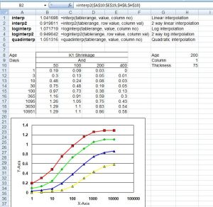
Interpolation functions