Today I found that some of my plotly functions were not working, and re-loading the pyxll files returned the message “could not import PySide6.Qtgui pyside6”. Searching for this problem I found:
It is necessary to clear cache files before reinstalling pyside6 other wise it will use previous cache files and the import error using continue to come.
But note that a following comment says that uninstalling and clearing the cache is not necessary.
Following the recent post on the Python lru_cache function (Python functools and the Fibonacci Sequence) I have had a look at using lru_cache in the 3DFrame-py spreadsheet. So far using lru_cache in this code has provided little to no speed improvement, but I did find changes to the basic code that resulted in very significant improvements. These are incorporated in the new release, that can be downloaded from:
See Installing 3DFrame-py for installation details, and details of other Python modules required. Also see Python and pyxll for details of the required pyxll package, including a coupon code for a 10% discount.
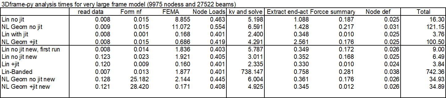
The most significant change is to the code to calculate beam fixed end actions under the applied loading. The original code allowed for beams with spring end releases at one or both ends, but for beams without end releases much simpler procedures are possible, and the new code applies the simplified procedures wherever possible. The processing time for a very large frame with different code and conditions is shown below:
The main conclusions are:
Total run time for linear analysis with “no jit” code was reduced by half, with the majority of the speed improvement in the code for Fixed End Moment Array (FEMA).
Using the Numba jit code, the old code was already fast, and this code was not updated.
For the analyses including non-linear geometric effects the total analysis times were almost the same for the new non-jit code, and the code with jit. The reasons for this are to be investigated.
One linear run used the “banded” solver. This was very slow, increasing the total solution time to over 12 minutes!
All the other runs used the PyPardiso solver, which is much faster than any of the Scipy solvers, but also has a further significant speed-up if an analysis is re-run without changing the stiffness matrix. This has the potential to speed up non-linear analyses, which will be investigated in future releases.
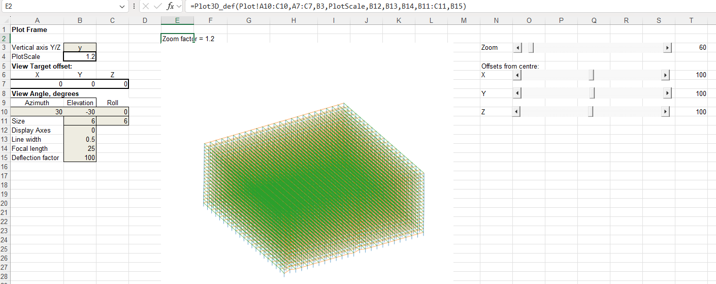
The other main change in the new code is that the VBA code to plot the frame in 3D has been replaced with Python code linking to my Plot3D function (see 3D plots with the latest Matplotlib). This has similar functionality to the VBA code but:
The Python code is very much faster. Redrawing the full frame for this large model with the VBA code took over 10 minutes. This is reduced to less than 1 second with Python.
The input data ranges are now selected automatically, and the plot re-draws automatically when anything is changed.
I have added slider bars to adjust the zoom ratio and the centre of view coordinates.
The full frame, with deflections magnified by 100 times:
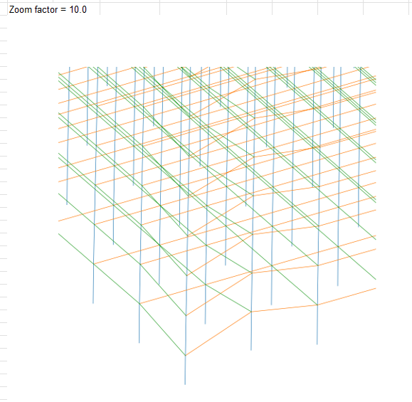
Zoom in and pan down to the front corner of the frame:
Increase the deflection factor to 200 x:
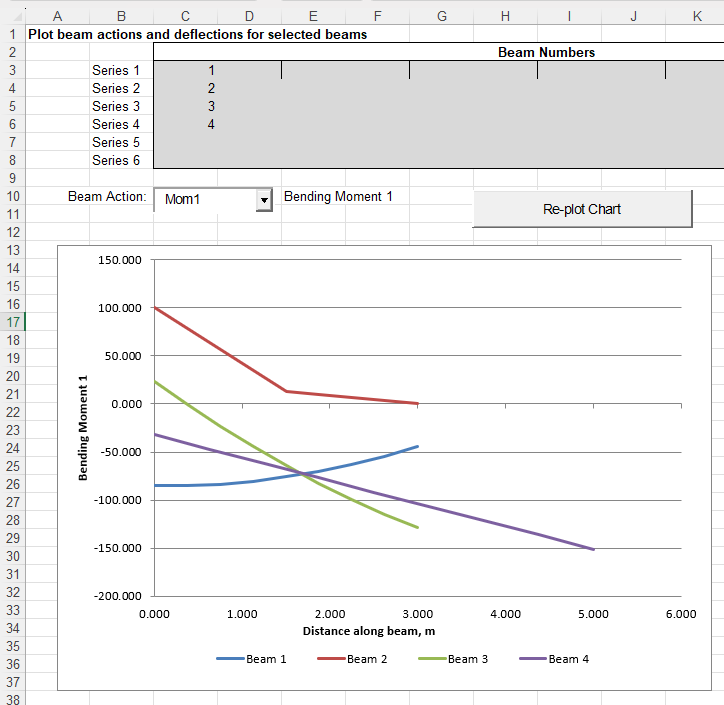
The graph to plot selected beam actions or deflections has also been updated (but currently still uses VBA):
Coincidentally, following the previous post, New Scientist’s regular brain teaser featured the iccanobiF Sequence, which is just like the Fibonacci Sequence, except that after adding the two previous numbers the digits of the results are reversed. Obviously the sequences are the same for single digit values, but following 5 and 8 the Fibonacci result is 13, and iccanobiF is 31.
The Python functools module has been around since 2006, so it’s not exactly new, but it is something I don’t currently use, but with potential to be useful.
This link: Functools module in Python provides details and examples of all the functions available, but this post will focus on the lru_cache function, which caches recent function results to speed up repeated calls with the same arguments. The example from the link calls a function to find the factorial of any input integer, and I had a look at that application here in 2022 (Python functools – cache and lru_cache), but an earlier post from the same site presents a similar function to calculate the Fibonacci Sequence: Python Functools – lru_cache(), which I have adapted to call from Excel with pyxll.
the Fibonacci sequence is a sequence in which each element is the sum of the two elements that precede it. The sequence begins: 0, 1, 1, 2, 3, 5, 8, 13, 21, 34, 55, 89, 144, …
The code below uses a simple recursive function to return the Fibonacci Number from any position in the sequence. It is followed by an alternative using a loop in place of the recursive function calls, then an alternative recursive function, modified to greatly reduce the number of calculation steps:
@xl_func()
@xl_arg('n', 'int')
def fibonacci(n):
    if n < 2:
        return n
    return fibonacci(n - 1) + fibonacci(n - 2)

@xl_func()
@xl_arg('n', 'int')
def fibonacci2(n):
    f1 = 1
    f2 = 1
    for i in range(2, n):
        f3 = f2+f1
        f1 = f2
        f2 = f3
    return f3

@xl_func()
@xl_arg('n', 'int')
def fibonacci9(n, a= 1, b=2):
    if n <= 2:
        return a
    else:
        return fibonacci9(n - 1, b, a+b)
Each of these functions has been modified with three alternative decorators:
Functools lru_cache: @lru_cache(maxsize=128)
Numba just-in-time compiler in “no python” mode: @njit
Numba with “parallel” enabled: @njit(parallel = True)
Results and execution times for the 12 alternative functions are shown below for input values (N) of 10 and 40:
All the options give the same results, but with widely different timing. For N = 10:
With the recursive function use of lru_cache slows down the results by about half. Both jit options are faster, with the parallel option doubling the speed compared with jit alone.
The loop function is about twice as fast as the plain recursive function, 5 times faster with lru_cache, and 3 to 4 times faster with jit.
The second recursive function is about twice as fast as the loop with no cache, similar with the cache, and very much slower than both of the other functions with either jit option.
For N = 40:
The recursive function with no cache is very slow, with the time being roughly proportional to the output Fibonacci number, rather than the input value.
The recursive function with lru_cache is about 240,000 faster, but the loop function with no cache is about 50% faster than that, and the recursive2 function is nearly 5 times faster again.
Use of lru_cache with the loop and recursive2 functions gives further significant speed increases, with recursive2 with lru_cache being over 3.5 million times faster than recursive without cache.
The jit functions with recursive are both only about 20 times faster than the function with no cache. With recursive2 they are both very much slower than the same function with no cache.
The loop function with jit on the other hand were 2.5 to 3.5 million times faster than recursive with no cache, and loop with jit+parallel was about equal fastest overall with recursive2 with lru_cache.
For the input shown above the numerical results are all identical, but for N = 93 or greater the result is greater than the maximum 64 bit integer, and the functions using either jit option return an incorrect result. Note that the values returned by all the other options are only accurate to machine accuracy, so they will also be wrong past the 15th significant figure.:
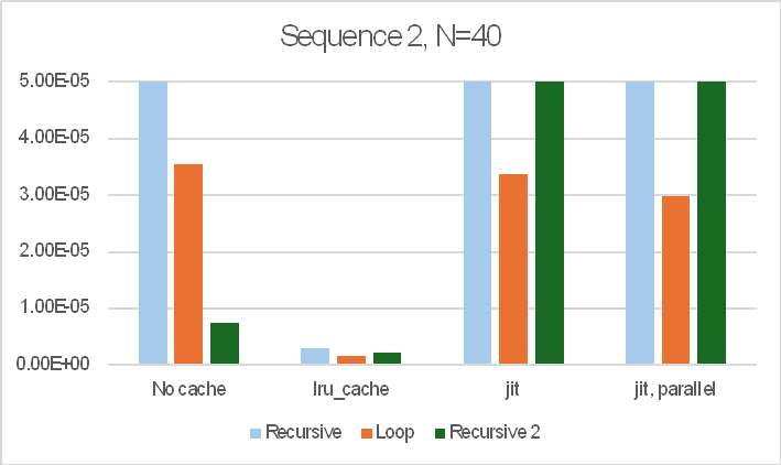
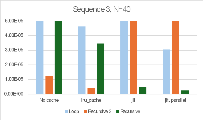
The sequence of operations also made a large difference to the results. The bar charts below show the results for three different sequences of the 12 functions:
Note that the bar charts are all cut off at 50 microseconds (5.0E-5 sec.) so that the relative performance of the faster options is visible. The recursive function with no cache took over 12 seconds in all cases.
In summary:
The recursive function with no cache was always very slow.
The best performer from the other options was highly variable, depending on the number of iterations required and the order the functions were called in, but the lru_cache function always gave good results and was often the fastest option.
The jit options were highly variable, sometimes being very fast, but in others being much slower than lru_cache, or the loop or recursive2 functions with no cache.
For real applications it would be worth looking at all the options in practice.