The Dome of Santa Maria del Fiore in Florence; new links

Earlier this year the on-line edition of National Geographic posted an article on:

Mystery of Florence’s Cathedral Dome May Be Solved

The wording of the article owes more to journalistic hyperbole than anything else, but it includes a link to an interactive 360 degree image of the cathedral interior of quite amazing detail.  The screenshot below shows a detail from the dome, but visit the link (about half way down) to view any other part of the cathedral interior in similar detail.

Duomo-1

Other links from this article include:

Redefining the Dome

An Interactive History of the Dome

The Secrets of the Florentine Dome

As we will see in this article, this great building site, challenging all of human knowledge at that epoch, was the locomotive provoking a scientific and technological revolution. Raising the great dome drew new horizons, which far beyond the construction of a building sent ripples and shockwaves of philosophical optimism to the great benefit of future generations.


Posted in Arch structures, Bach, Dome Structures, Newton | Tagged , , , | Leave a comment

Evaluating text – update

One disadvantage of the spreadsheet style interface is that even simple formulae are difficult to check.  For instance, the deflection of a cantilever loaded at the end is given by:
F*L^3/(3*E*I)
which is much easier to read than the Excel version:
=B31*B32^3/(3*B33*B34)
It is possible to allocate names to the spreadsheet cells, but this rapidly becomes cumbersome if there are more than a few formulae, or if a formula is repeated with different data.

The spreadsheet Eval2.xlsb overcomes these problems by allowing the evaluation of formulae entered as text:

Eval2-2-1

In the example above, the text formula in Cell A29 is evaluated using the values listed in the range A31:B34.  The Eval function also has the option to return a text string with the variable names replaced with values, as seen in Cell D31.

The original version of this function had the disadvantage that short variable names might corrupt longer names, or function names, that included the same characters.  For instance a variable “a” would result in “ab” or “tan” having their a characters replaced by the value of a.  I have now re-written the function, using the VBA scripting dictionary, so that all variable names only apply to a string of the same length.  The new function, including full open source code, may be downloaded from the link below.  Links are also provided to other spreadsheets using the Eval function.

The screenshot below shows an example of the use of the new version with a variable name that would previously have caused an error.  Note also that the range specifying the variable names and values may now be entered as a single range of two adjacent columns, or two separate ranges.

Eval2-2-2

The Evala function returns an array of values with evaluation of a single formula.  In the example below the formula for K2 is evaluated for a range of values of t and th:

Eval2-2-3

The Eval-Integration spreadsheet (included in the Eval2.zip download) includes a number of functions for numerical integration of any function of a single variable, including the Tanh-Sinh method (based on a function provided by Graeme Dennes), and Gauss-Kronrod Quadrature, using the Alglib library:

Eval2-2-4

The new version has also been included in the Units4Excel spreadsheet, allowing unit aware evaluation of any formula, using a wide range different units:

Eval2-2-5


Posted in AlgLib, Excel, Maths, Newton, Numerical integration, UDFs, VBA | Tagged , , , , , , , | 5 Comments

Reinforced Concrete – ULS capacity under combined axial load and biaxial bending

I have modified the ULS Design Functions spreadsheet, last presented here, to analyse sections subject to bi-axial bending, and non-symmetrical sections.  The new version makes use of the routines for splitting any section defined by XY coordinates into trapezoidal layers, described here.  The new version (ULS Design Functions-biax.xlsb) has been added to the zip file along with the previous version, and can be downloaded from ULS Design Functions.zip, including full open source code.

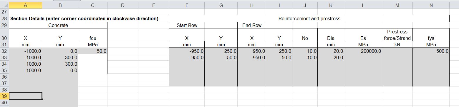
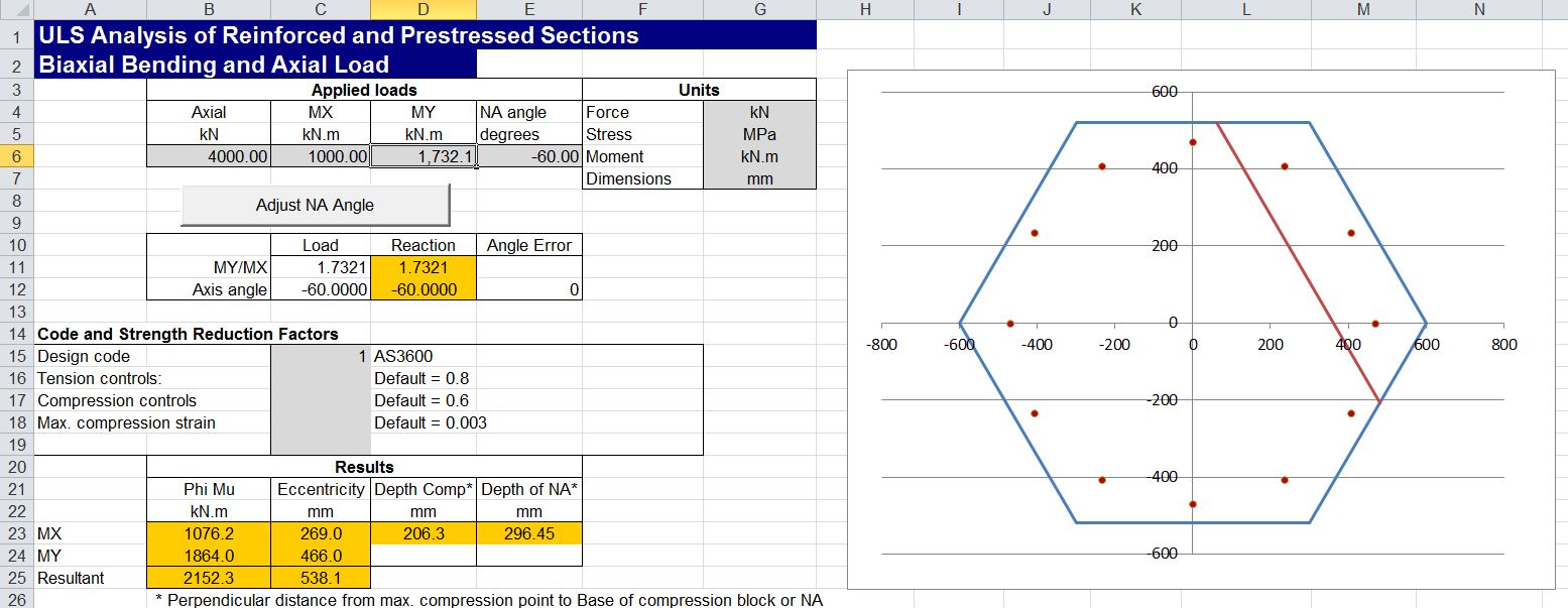
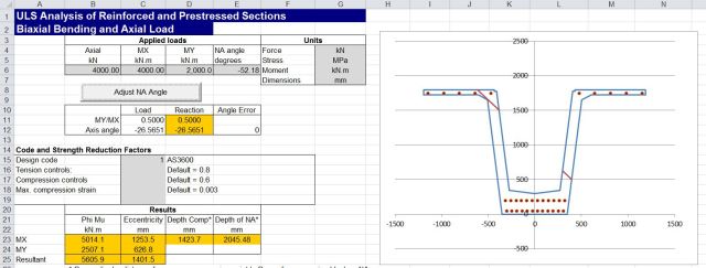
Input and results for a wide rectangular section, subject to bi-axial bending and axial load, are shown in the screenshot below:

Biax-1

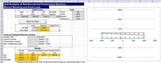
The direction of the applied moment is defined by MX and MY, then the Neutral Axis angle is adjusted so that the reaction force and moments are in equilibrium with the applied loads, by clicking the “Adjust NA Angle” button.

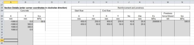
The concrete section is defined by XY coordinates of each corner, listed in a clockwise direction, and the reinforcement is defined in layers, by entering the coordinates of the start and end of each layer:  For each layer the number of bars and bar diameter are defined, together with the steel properties for the first layer, and any subsequent layer with different properties.  It is also possible to specify a prestress force for any layer.

Biax-2

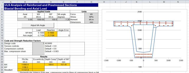
The hexagonal section shown below demonstrates that for a symmetrical section the angle of the resultant moment axis is parallel to the Neutral Axis angle, as would be expected:
Biax-3

It is possible to define any complex shape, such as the precast Super-T bridge girder shown below:
Biax-T1

It is also possible to define shapes with internal voids, as shown below, by listing the corners of the void in the anti-clockwise direction.  In this case the line must be continuous from start to end, and the connection between the outer line and the void must be made with two separate lines, with a very small separation, so that separate lines do not overlap or cross at any point.  See the example in the download file for more details.
Biax-T2

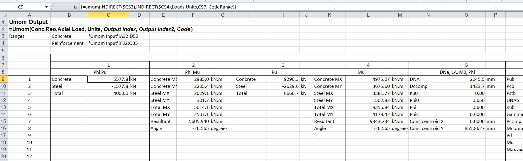
More detailed output data is provided on the “UMom Out” sheet, in a similar format to the earlier version.
Biax-6

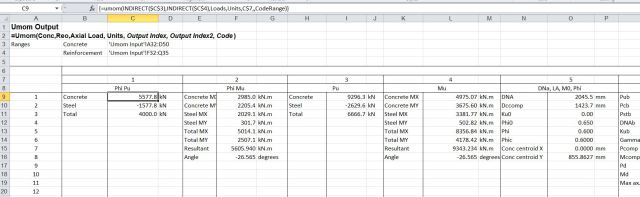
The analysis is carried out by two user defined functions (UDFs), UMom and UMomA.  UMom provides the detailed output shown above for a single set of applied loads.  UMomA returns any one of the available output values for a range of applied axial loads, and a single value or range of Neutral Axis directions.  Both functions return an array of values, and must be entered as an array function, as described at Using Array Functions and UDFs.

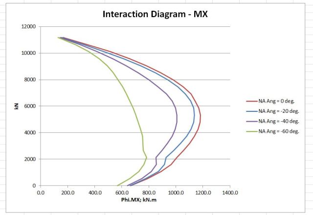
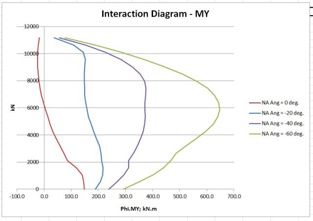
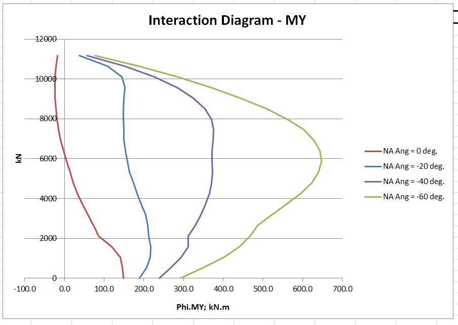
Use of the UMomA function allows the rapid generation of interaction diagrams, as shown in the screenshots below:
Biax-7


Biax-8

Posted in Beam Bending, Concrete, Excel, Newton, UDFs, VBA | Tagged , , , , , , | 13 Comments

Melanie Safka

Melanie Safka is touring Australia this month, which prompted me to look up some of her old songs on YouTube – I’d forgotten how good she was:

And something more recent, London in 2009:


Posted in Bach | Tagged | 1 Comment

Data Transfer to Python – Update

As noted in the comments here, the main bottleneck in the Python matrix solver functions presented recently was not in the data transfer from Excel, but rather in the creation of the Numpy arrays for very long lists of short lists (see this Stackoverflow thread for more details of the background).  It seems there is a substantial time saving in converting the long array into 1D vectors, which can be converted into Numpy arrays very much more quickly.  The VBA code below converts a 3D array of any length (up to the maximum allowed in Excel) to 3 vectors.

Function Vectorize(x As Variant, x_1 As Variant, x_2 As Variant, x_3 As Variant) As Long
Dim nr As Long

nr = x.Rows.Count
x_1 = x.Resize(nr, 1).Value2
x_2 = x.Offset(0, 1).Resize(nr, 1).Value2
x_3 = x.Offset(0, 2).Resize(nr, 1).Value2
Vectorize = nr
End Function

To transfer these vectors to Python, via ExcelPython, the PyObj function must be used:

Set x = Range("SSA")  ' Excel range with 500500 rows and 3 columns
n = Vectorize(x, x_1, x_2, x_3) 'Convert range values to 3 vectors
' Create ExcelPython objects for transfer to Python
Set x_1 = PyObj(x_1, 1)
Set x_2 = PyObj(x_2, 1)
Set x_3 = PyObj(x_3, 1)

In Python the three vectors are converted to Numpy arrays:

def xl_getnpvect(x_1, x_2, x_3):
    timea = np.zeros(4)
    timea[0] = time.clock()
    x_1 = np.array(x_1)
    timea[1] = time.clock()
    x_2 = np.array(x_2)
    timea[2] = time.clock()
    x_3 = np.array(x_3)
    timea[3] = time.clock()
    return timea.tolist()

The table below compares the data transfer and conversion times using this method on an Excel range of 500500 rows x 3 columns, with the same operation using a 2D variant array.

XLpyMatrix3-0

The times for solution of a large sparse matrix system (10945×10945 matrix), using the new vector transfer routine, are shown below:
XLpyMatrix3-1

The data transfer and array creation times are now a relatively small proportion of the total solution time, even for the iterative solver with a solve time of only 0.28 seconds.

Posted in Arrays, Excel, Frame Analysis, Link to Python, NumPy and SciPy, VBA | Tagged , , , , , | 4 Comments