Browsing the Plus Magazine site recently, I was struck the proof of Pythagoras’ Theorem shown in the animation below:

Not just because it is an elegant proof, but also because of the author, the 20th President of the United States, James Garfield.

Browsing the Plus Magazine site recently, I was struck the proof of Pythagoras’ Theorem shown in the animation below:
Not just because it is an elegant proof, but also because of the author, the 20th President of the United States, James Garfield.
The code described in the previous post includes a Python function that rotates 3D coordinates by an angle defined with two vectors, using Rodrigue’s Rotation. I have now added this function to the IP2_py spreadsheet, where it is used in the original application (fitting a circular arc to 3D data points), and also in the PView user defined function (UDF), to generate a perspective projection of any 3D framework. The new spreadsheet and associated Python code may be downloaded from:
As well as the new functions, the update includes:
Examples of the new PView and Fit_Circ3D functions are shown in the screenshots below:


As for the previous application, to use the spreadsheet:
Following a comment at update-to-glob_to_loc3-and-loc_to_glob3-functions, I have modified the Python code at the linked site, so it can be run from Excel, via xlwings. The spreadsheet described below, and the associated Python code, can be download from:
The original code and background information can be found at: Fitting a Circle to Cluster of 3D Points. The code performs the following functions:
To simplify the process as far as possible, I have converted the code to two user-defined functions (UDFs) that can be called from Excel, using xlwings, to generate the cloud of points, and to return the coordinates of a series of points along the best fit circle, or along an arc extending over the range of the data. This data is then plotted in Excel, using xy charts.
Typical spreadsheet input and output are shown in the screen shots below:
The Points_by_ang function generates points along an arc of the specified circle, with random 3D offsets of magnitude determined by the k factor. The input data in the example is the same as is hard coded in the original Python code. The Fit_circ3D functions returns 3D coordinates along the best fit arc or circle (or alternatively other results, as defined by the “out” value). Note that if the number of generated points is changed from 100, the range must be adjusted in the fit_Circ3D function, so that all of the input data range contains real numbers, not #N/A# or blank cells.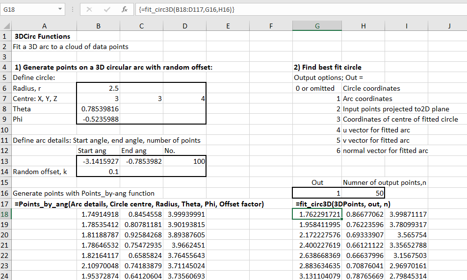
The best fit circles, projected to the XY, XZ and YZ planes, are shown below: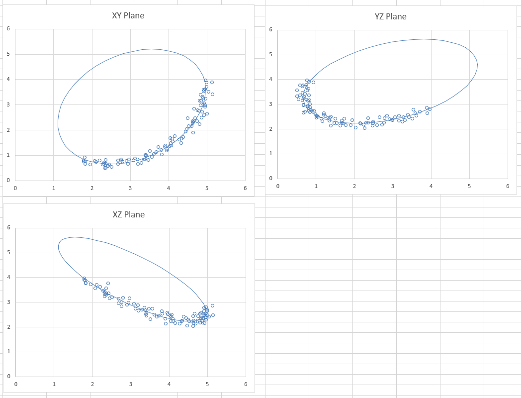
The Matplotlib results from the original code are very similar: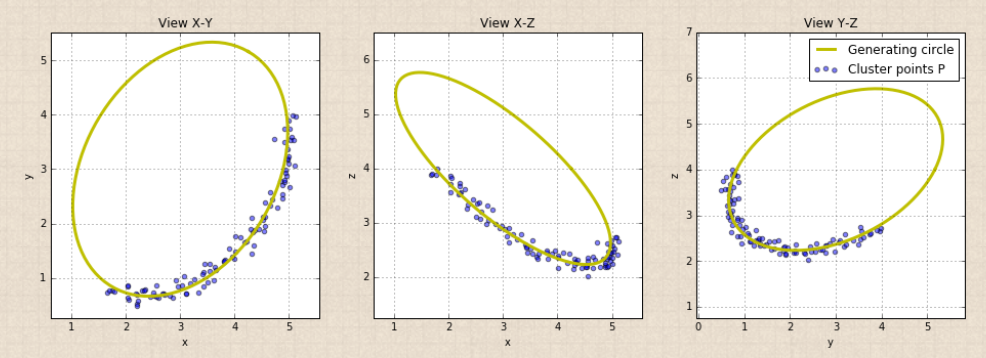
Changing the input data, the graphs automatically re-draw to show the new results: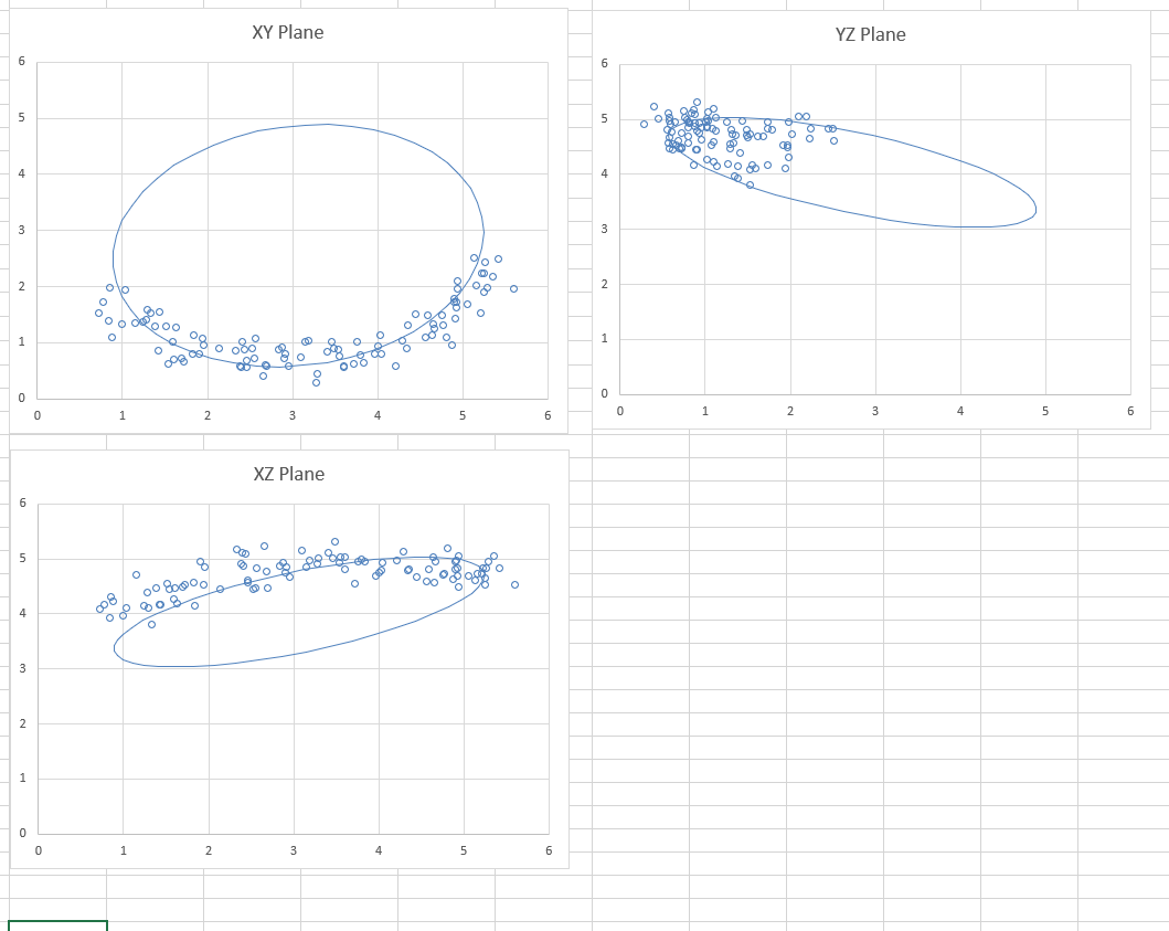
To use different input points (either generated from another source, or real survey data) simply paste the data anywhere in the spreadsheet, and adjust the “3DPoints” range in the Fit_circ3D function, and the chart data ranges for the input data.
To use the spreadsheet:
A cubic spline provides a good approximation to a smooth curve, and alternative versions are available for free download (see Daily Download 22: Splines and Curves, Update to AL-Spline-Matrix, and xlwSciPy 1.09 – update for xlwings 0.10 and Scipy 0.18.1), but if a curve has a sharp change of direction a single cubic spline will deviate significantly from the required values near the change. An example of curves where this is a problem is a reinforced concrete moment-curvature diagram, which has sharp changes of slope at the cracking moment, and also at the reinforcement yield point.
To deal with curves of this sort, I have added an MSplineA user defined function (UDF) to the CSpline2 spreadsheet, which may be downloaded (including open-source code) from:
This function allows a curve to be divided into any number of segments, each of which may be either linear or cubic splines. Input and output details, and a typical example are shown in the screen shots below:

Required input ranges are the X and Y values of the input data, a list of spline segments, listing the last node number of each segment, the spline type to be applied (1 = linear or 3 = cubic), and end curve or slope details for cubic splines, and the X values where interpolation is required:
Output for this example is shown below:
Looking more closely at the region near the cracking moments it can be seen that the MSplineA function has given a good approximation to the input values, whereas a single cubic spline deviates significantly:
In June last year I posted a link to a Jeremy Corbyn speech on the topic of building bridges, not walls.
Here are a couple of (more poetic) links on the same topic.
The first is from Anaïs Mitchell. This song was written over 10 years ago, as part of the folk opera Hadestown, and the word are those of Hades, Lord of the Underworld:
An interesting interview with Anaïs Mitchell from 2016:
The singer-songwriter Anaïs Mitchell grew up on a sheep farm in semirural Vermont to a soundtrack of folk ballads and protest music. As a child, she believed that “if you could just write a song good enough, you could change the world.”
That belief has never quite left her. She is testing it in her first musical, the theatrically frisky and musically daring “Hadestown,” a version of the Orpheus myth retold in the American vernacular, which just opened at New York Theater Workshop.
…
One of Mr. Page’s songs will send a shiver for anyone following the presidential election: “Why We Build the Wall.” Though Ms. Mitchell wrote it a decade a ago, the song has taken on the uncanny echo of Donald J. Trump’s remarks on the campaign trail. Ms. Mitchell is unsurprised. “Political leaders will always invoke that image when it serves them,” she said, “because it appeals at a visceral level to people who feel scared.”
Ms. Mitchell is not scared, and she plans to keep writing — for the concert stage and the theatrical one. The Orpheus-like part of her insists on it. “Whether or not you can change the world with a song, you’ve still got to write the song,” she said. “You still have to try.”
Full interview at The New York TimesNew York Times.
The second is from Melanie Safka, singing “Close To it All” at a live performance in 1971:
