A convenient way to create an animation in Excel is to create on-sheet formulas or user defined functions to generate the required data, then use VBA to iterate through the range of input values so that the chart or image will update for each iteration. A problem with this approach is that often the image will not redraw, while the code is running.
Searching for a solution to this problem, there were surprisingly few discussions on this problem, and most of those I did find I couldn’t get to work, but eventually I found a solution using ActiveWindow.SmallScroll, which has the twin benefits of being very simple, and obvious how it works. Example VBA code is shown below.
Edit 2 Dec. 2021: Modifications to the code for generating the images resulted in very short cycle times, so I added some code to “sleep” between cycles, so the cycle time was at least 1 second. Sleep is a Windows function, so has to be “declared” at the top of the code module. I have also added code to time each iteration, so the sleep period is reduced as the time for generating the image increases. An added benefit of this code is that it has removed the white screen flashing between each iteration, so the resulting video is much smoother.
#If VBA7 Then ' Excel 2010 or later
    Public Declare PtrSafe Sub Sleep Lib "kernel32" (ByVal Milliseconds As LongPtr)
#Else ' Excel 2007 or earlier
    Public Declare PtrSafe Sub Sleep Lib "kernel32" (ByVal Milliseconds As Long)
#End If

Sub Zoomin()
Dim Startfact As Double, inc As Double, steps As Long, Fact As Double
Worksheets("Sheet4").Activate
With Application.ActiveSheet
    Startfact = Range("Start").Value
    inc = Range("Factor").Value
    steps = Range("steps").Value

    Fact = Startfact
    For i = 1 To steps
        STime = Timer()
        Range("Scale").Value = Fact
        Range("Iteration") = i
        ActiveWindow.SmallScroll down:=1
        ActiveWindow.SmallScroll up:=1
        Fact = Fact * inc
        TimeDiff = (Timer() - STime) * 1000
        If TimeDiff < 950 Then
            Sleep (1000 - TimeDiff)
        Else
            Sleep (50)
        End If
    Next i
End With
End Sub
An example animation generated with this routine (plus a Python user defined function to generate the images) is shown below. More details of the code for generating the images will be provided in a later post:
Zoom in x2 24 times
With the faster image generation I have added a second video zooming in 48 times, with a final magnification of 2.8E+14 times, which is about as far as you can get with the resolution allowed with 64 bit float values:
Following some recent comments Graeme Dennes has released the latest version the Tanh-Sinh Quadrature spreadsheet with some corrections to the test function documentation.
For more information on the last major release see Numerical Integration With Tanh-Sinh Quadrature v 5.0. For more background information and numerous examples search this site for Tanh-Sinh, or select Numerical Integration from the categories drop down.
As always, if you have any questions or comments, please leave a comment below.
Every so often I check YouTube to see what new old music has been posted, and today I found:
Haitian Fight Song, here played by Danny Thompson in Norway in 1968
and Bert Jansch and Danny Thompson playing Thames Lighterman (great pictures as well as great music):
Bert Jansch composition. Recorded at the BBC for John Peel’s Night Ride, broadcast Dec 18, 1968. Apologies for poor sound quality: taken from 50 year old 1/4″ 4-track mono tape running at 3 3/4 ips. The title refers to Pentangle roadie Bobby Cadman, whose previous occupation had been Thames Lighterman. Bert’s song “One For Jo” is also about him, addressed to Bobby’s wife.
The pyxll documentation has many examples of plotting in Excel using Matplotlib and other packages, but I find the multiple options confusing and hard to follow, so this post works through the examples in the Matplotlib Users Guide tutorial. The sample spreadsheet and python code can be downloaded from:
Note that all the examples below were taken from the manual for Release 2.0.2. The current release is 3.4.3, and includes several additional examples, and considerably more background information.
The first example plots a simple line graph using hard coded data. I have added a modified version that will transfer the data from a selected row on the spreadsheet.
import matplotlib.pyplot as plt
from matplotlib import colors

import pyxll
from pyxll import xl_func, xl_arg, xl_return
from pyxll import  plot

@xl_func
def MPLTute_1():
    # Create the figure
    fig = plt.subplots()[0]
    # Plot the data
    plt.plot([1,2,3,4])
    plt.plot([0,2,4,6])
    plt.ylabel('some numbers')
    # Display the figure in Excel
    plot(fig)

@xl_func
@xl_arg('data','float[]')
def MPLTute_1a(data):
    fig, ax = plt.subplots()
    ax.plot(data)
    ax.set(ylabel='some numbers')
    plot(fig)
The first function follows the code in the tutorial as closely as possible, with the addition of a second plotted line. The second function, in addition to reading the data to be plotted from the spreadsheet, follows the coding used in the pyxll examples more closely.
The next example plots XY data, read from the spreadsheet as a list of lists. The string ‘ro’ plots the line as red circles for each data point (see the manual for details):
Function 3 plots 3 lines, each with a different format string. The lines are hard coded functions of the range “t”. The lines are created with a single .plot, as a sequence of 3 sets of X values, Y values, line format string:
Function 4 plots one of the lines from the previous example, but instead of using a single string to format the line, a dictionary is passed from the spreadsheet, allowing multiple format properties to be specified:
@xl_func
@xl_arg('props','dict<str, var>')
def MPLTute_4(props):
    x = np.arange(0., 5., 0.2)
    y = x**2
    fig, ax = plt.subplots()
    ax.plot(x, y, **props)
    plot(fig)
The spreadsheet includes a list of available properties, but see the manual for full details:
Function 5 plots a histogram, using the plt.hist method:
@xl_func
def MPLTute_5():
    np.random.seed(19680801)
    mu, sigma = 100, 15
    x = mu + sigma * np.random.randn(10000)

    fig, ax = plt.subplots()
    # the histogram of the data
    # Changed from the tutorial example: "n, bins, patches = plt.hist(x, 50, normed=1, facecolor='g', alpha=0.75)"
    # because use of normed now raises an error.
    n, bins, patches = plt.hist(x, 50, density=1, facecolor='g', alpha=0.75)

    plt.xlabel('Smarts')
    plt.ylabel('Probability')
    plt.title('Histogram of IQ')
    plt.text(60, .025, r'$\mu=100,\ \sigma=15$')
    plt.axis([40, 160, 0, 0.03])
    plt.grid(True)

    plot(fig)
The comment noting the change from the code in the tutorial refers to the document for Release 2.02. The current tutorial (Release 3.4.3) has been corrected.
Function 6 illustrates the addition of text and graphics to the graph:
Finally Functions 7 and 7a illustrate the use of different axis types, and returning multiple graphs from a single function:
@xl_func
@xl_arg('scaletype', 'int')
def MPLTute_7(scaletype):
    fig, ax = plt.subplots()
    from matplotlib.ticker import NullFormatter # useful for `logit` scale
    # Fixing random state for reproducibility
    np.random.seed(19680801)
    # make up some data in the interval ]0, 1[
    y = np.random.normal(loc=0.5, scale=0.4, size=1000)
    y = y[(y > 0) & (y < 1)]
    y.sort()
    x = np.arange(len(y))
    # plot with selected axes scale
    if scaletype == 1:
        # plt.figure(1)
        # # linear
        # plt.subplot(221)
        plt.plot(x, y)
        plt.yscale('linear')
        plt.title('linear')
        plt.grid(True)
        # log
    elif scaletype == 2:
        # plt.subplot(222)
        plt.plot(x, y)
        plt.yscale('log')
        plt.title('log')
        plt.grid(True)
        # symmetric log
    elif scaletype == 3:
        # plt.subplot(223)
        plt.plot(x, y - y.mean())
        plt.yscale('symlog', linthreshy=0.01)
        plt.title('symlog')
        plt.grid(True)
        # logit
    elif scaletype == 4:
        # plt.subplot(224)
        plt.plot(x, y)
        plt.yscale('logit')
        plt.title('logit')
        plt.grid(True)
    else:
        return 'scaletype must be between 1 and 4'
    # Format the minor tick labels of the y-axis into empty strings with
    # `NullFormatter`, to avoid cumbering the axis with too many labels.
    plt.gca().yaxis.set_minor_formatter(NullFormatter())
    # Adjust the subplot layout, because the logit one may take more space
    # than usual, due to y-tick labels like "1 - 10^{-3}"
    # Not required, Excel version returns only 1 chart
    # plt.subplots_adjust(top=0.92, bottom=0.08, left=0.10, right=0.95, hspace=0.25,
    # wspace=0.35)

    plot(fig)


@xl_func
def MPLTute_7a():
    # Multiplot version
    fig, ax = plt.subplots()
    from matplotlib.ticker import NullFormatter # useful for `logit` scale
    # Fixing random state for reproducibility
    np.random.seed(19680801)
    # make up some data in the interval ]0, 1[
    y = np.random.normal(loc=0.5, scale=0.4, size=1000)
    y = y[(y > 0) & (y < 1)]
    y.sort()
    x = np.arange(len(y))
    # plot with various axes scales

    fig = plt.figure(1)
    # # linear
    plt.subplot(221)
    plt.plot(x, y)
    plt.yscale('linear')
    plt.title('linear')
    plt.grid(True)
    # log
    plt.subplot(222)
    plt.plot(x, y)
    plt.yscale('log')
    plt.title('log')
    plt.grid(True)
    # symmetric log
    plt.subplot(223)
    plt.plot(x, y - y.mean())
    plt.yscale('symlog', linthreshy=0.01)
    plt.title('symlog')
    plt.grid(True)
    # logit
    plt.subplot(224)
    plt.plot(x, y)
    plt.yscale('logit')
    plt.title('logit')
    plt.grid(True)

    # Format the minor tick labels of the y-axis into empty strings with
    # `NullFormatter`, to avoid cumbering the axis with too many labels.
    plt.gca().yaxis.set_minor_formatter(NullFormatter())
    # Adjust the subplot layout, because the logit one may take more space
    # than usual, due to y-tick labels like "1 - 10^{-3}"
    plt.subplots_adjust(top=0.92, bottom=0.08, left=0.10, right=0.95, hspace=0.25,
    wspace=0.35)

    plot(fig)
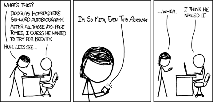
Today it was announced that Facebook, the meta company that owns Facebook, was going to be renamed “Meta”, which reminded me of an xkcd episode from 10 years ago:
This is the reference implementation of the self-referential joke